What’s New in Astro Python SDK 1.1: Data-Driven Scheduling, Dynamic Tasks, and Redshift Support

In case you’re not already writing Airflow data pipelines with the Astro Python SDK, we’ve just released some compelling features for data engineers and data scientists in the Python SDK 1.1:

• Data-driven scheduling using Dataset objects in Airflow 2.4
• Dynamic Task Templates that use Dynamic Task Mapping (Airflow 2.3+)
• Support for Redshift

Schedule Your DAGs When Upstream Data Is Ready

One of the showcase features of Airflow 2.4 is the Dataset object, a global data object that unlocks a whole new world of authoring data workflows. Now you can write smaller, modular directed-acyclic graphs (DAGs) that communicate with and trigger each other via Datasets. Let’s look at a simple example of data-driven scheduling and then explore the many benefits of writing DAGs that follow this paradigm.

Consider the straightforward ELT pipeline in the Astro Python SDK GETTING_STARTED example, in which we are loading data from an S3 file store to a Snowflake data warehouse, and then performing some transformations in the warehouse.

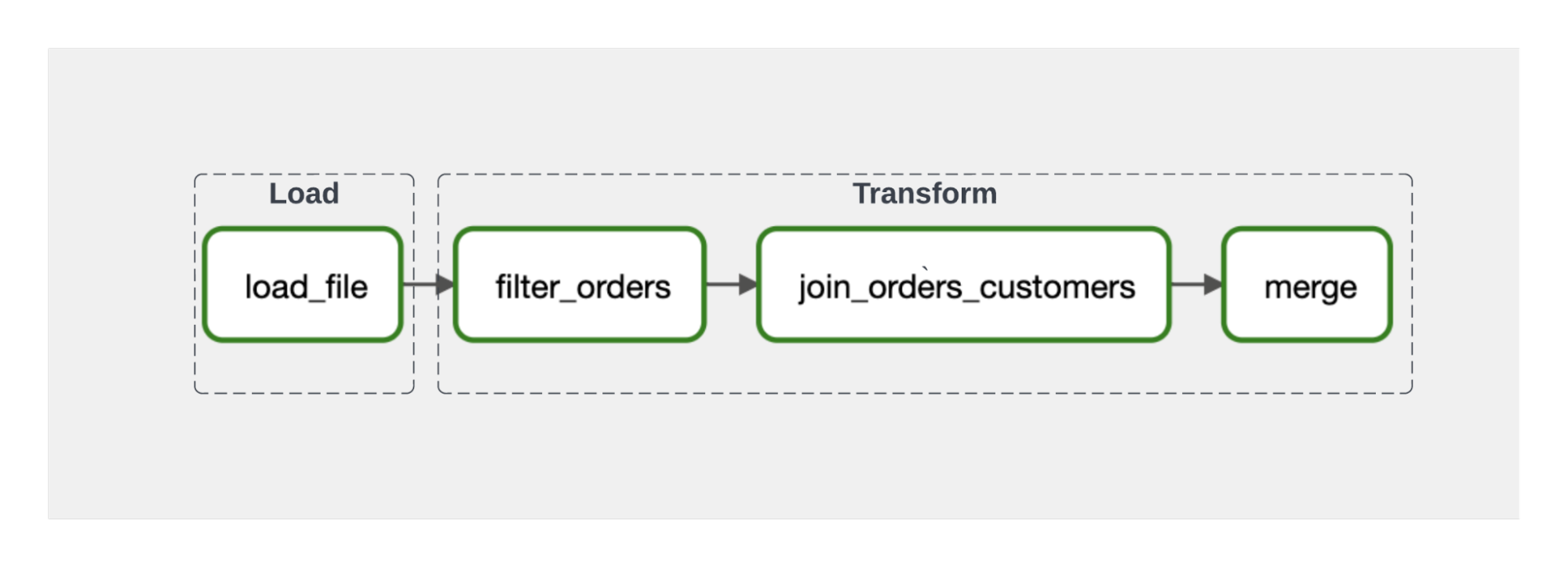Figure 1: A simple ELT DAG in which we use task dependencies to ensure that upstream tasks have finished preparing data that downstream tasks require.

We accomplish these steps in a single DAG, where we begin our transformation step only after the load has finished, using a task dependency that the SDK infers from introspecting our DAG code. Instead of using task dependencies as a proxy for data dependencies, with Airflow 2.4 and SDK 1.1 we can now model the data dependencies directly. Specifically, the SDK File and Table classes inherit from the Airflow Dataset class, so you can schedule your DAGs to trigger the moment that upstream data is ready.

Under this data-driven paradigm, we’ll want to re-factor our single DAG into two, which communicate with each other via a Table object. In the first DAG (below), the data-producing DAG, we declare a Table object, orders_table, as we normally would with the Python SDK. Nothing new going on here since SDK 1.0:

orders_table = Table(name=SNOWFLAKE_ORDERS, conn_id="snowflake_default")

dag = DAG(
   dag_id="astro_producer",
   start_date=START_DATE,
   schedule_interval='@daily',
   catchup=False,
)
with dag:
   orders_data = aql.load_file(
       input_file=File(path=S3_FILE_PATH + '/orders_data_header.csv',  conn_id=S3_CONN_ID),
       output_table=orders_table,
   )

Here’s where the magic happens: In our second DAG (below), the data-consuming DAG, we again declare a Table object, orders_table_demo, using the same data warehouse table name and connection information. Note: You can assign a different variable name to this Table object compared to what you called it in the data-producing DAG. All that matters is that the underlying table name and database connection are the same.

Then, we set a schedule parameter for the DAG to include the orders_table_demo object. Note: You can schedule a DAG to proceed based on the completion of any number of File and Table objects.

The Python SDK introspects your code to determine when processing on the Table object completes. You don’t need to explicitly determine which task to set the outlets parameter on, as you would with using Dataset objects without the SDK, described in Datasets and Data-Aware Scheduling in Airflow.

orders_table_demo = Table(name=SNOWFLAKE_ORDERS, conn_id="snowflake_default")

dag = DAG(
   dag_id="astro_consumer",
   schedule=[orders_table_demo],
   start_date=START_DATE,
   catchup=False,
)
with dag:

   # create a Table object for customer data in our Snowflake database

   customers_table = Table(name=SNOWFLAKE_CUSTOMERS,conn_id=SNOWFLAKE_CONN_ID)

   # filter the orders data and then join with the customer table

   joined_data = join_orders_customers(filter_orders(orders_table_demo),customers_table)

   # merge the joined data into our reporting table, based on the order_id .

   # If there's a conflict in the customer_id or customer_name then use the ones from

   # the source_table

   reporting_table = aql.merge(
       target_table=Table(
           name=SNOWFLAKE_REPORTING,
           conn_id=SNOWFLAKE_CONN_ID,
       ),
       source_table=joined_data,
       target_conflict_columns=["order_id"],
       columns=["customer_id", "customer_name"],
       if_conflicts="update",
   )

In the Airflow UI, you’ll now find a “Datasets” tab on the home screen. This tab shows how your DAGs and Datasets are connected.

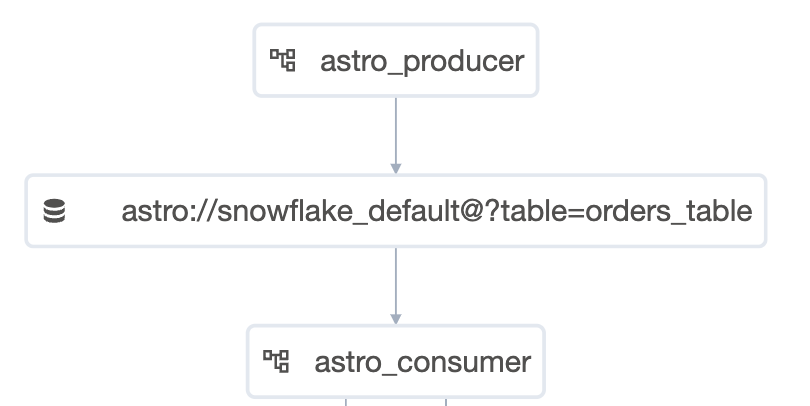Figure 2: Airflow 2.4 depicts data dependencies among DAGs. Here, when the astro_producer DAG finishes creating the orders_table Table object, the completion of this table triggers the astro_consumer DAG.

Since the Dataset object gives us true data-driven scheduling of DAGs, we no longer have to use workarounds to manage our data dependencies. Historically, these workarounds included:

Workaround	Drawbacks
Monolithic DAGs: Organize tasks and task groups in a large DAG to model the data dependencies as dependencies among tasks and task groups.	Execution of downstream DAGs will be delayed because your task groups need to wait for the longest-running task in an upstream task group. In other words, introducing a single long-running task can delay the delivery of all the data products from the workflow. (See our blog on micropipelines for more information.) Code is difficult to maintain because DAGs are large.
Sensors: Separate tasks into multiple DAGs that use sensors for scheduling when upstream data is ready.	Sensor polling occupies a worker node and burns up CPU cycles, unless you’re using deferrable operators. Additional code is required to implement sensors. Execution of downstream DAGs will be delayed due to interval of sensor polling.
Timers: Set time intervals on downstream DAGs to allow upstream DAGs to finish.	Execution of downstream DAGs will be delayed because your scheduling intervals will need to be set conservatively large to allow upstream DAGs to finish. Code is difficult to maintain when there are multiple upstream dependencies. DAGs will be brittle if an upstream process takes longer than expected.

While the data dependency depicted in the simple ELT example is trivial, you can imagine or have likely witnessed first hand how complicated real-life data dependencies can be, when many downstream tasks are each dependent on many upstream tasks to prepare data: the dreaded many-to-many relationship. We describe these complexities more in our recent blog on micropipelines.

Now that you can use data-driven scheduling to decompose your DAGs into more modular Python files, your new DAG authoring style will afford you a number of benefits:

• Data as a product: Teams that understand the data sources best can extract, load, cleanse, and publish data for other teams to transform further to meet the needs of their business-specific use cases. In other words, you can use Datasets as the foundational element of a data mesh architecture.
• Enhanced collaboration among teams: With modular DAGs, data practitioners with different types of expertise can build DAGs in their language of choice – e.g., Python or SQL – to publish Datasets, enabling teams to loosely couple their workflows. Compare the modular DAG paradigm to monolithic DAGs, where different types of practitioners would need to collaborate in a single, large DAG in the same programming language.
• Increased maintainability of DAGs: Compared to monolithic DAGs, modular DAGs will be easier to understand and modify over time, decreasing your risks for deploying updates to your pipeline code.
• Increased runtime efficiency: Data-driven scheduling using Datasets will be faster than time-driven scheduling since the data-driven DAG will be triggered exactly when any upstream data dependencies are satisfied. Moreover, you can deliver business-critical data on its own more timely schedule (e.g. daily), since it can be run separately from other less time-critical pipelines.

Create Tasks While Your DAG Is Running

Airflow 2.3 gave us dynamic task mapping, in which DAGs can generate parallel tasks at runtime. Astro Python SDK 1.1 brings this capability to SDK operators, including the load_file capability. In other words, your DAGs can spawn task instances for loading files, where your DAG doesn’t know how many and which files to load until it actually runs.

From the SDK library of examples, below you’ll see an excerpt that demonstrates how you can load files from a cloud store following the MapReduce() paradigm. For dynamic tasks, you pass function parameters through the partial() and expand() functions according to these criteria:

• partial(): This function passes any parameters that remain constant across all mapped tasks that are generated by expand().
• expand(): This function passes the parameter or parameters that you want to map on. A separate, parallel task will be created for each input.

from astro.files import get_file_list
from astro.sql.operators.load_file import LoadFileOperator as LoadFile

with DAG(
   dag_id="example_dynamic_task_template",
   schedule_interval=None,
   start_date=datetime(2022, 1, 1),
   catchup=False,
) as dag:
   LoadFile.partial(
       task_id="load_gcs_to_bq",
       output_table=Table(
           metadata=Metadata(
               schema=ASTRO_BIGQUERY_DATASET,
           ),
           conn_id=ASTRO_GCP_CONN_ID,
       ),
       use_native_support=True,
   ).expand(input_file=get_file_list(path=GCS_BUCKET, conn_id=ASTRO_GCP_CONN_ID))

In this example, get_file_list – also new to SDK 1.1 – retrieves a list of files from the cloud storage bucket. Then, the expand function creates a load_gcs_to_bq task instance for each of the file names retrieved. The partial function just specifies parameters that remain constant for each file-loading task instance.

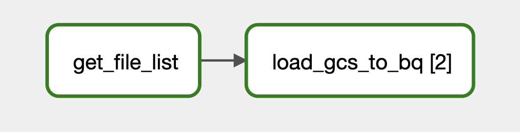Figure 3: In the Airflow UI Graph view for a DAG using dynamic task mapping (or dynamic task templates in the case of the Astro Python SDK), you’ll see mapped tasks with a set of brackets []. The number in the brackets shows how many mapped instances were created.

For a simple case – where there’s just two files in our bucket storage – we end up with two mapped instances of our dynamic task load_gcs_to_bq in the Airflow UI Graph view.

Build DAGs on Redshift

Astro Python SDK 1.1 adds Redshift to the list of supported data warehouses, along with Snowflake, Google BigQuery, and Postgres. For the load_file operation from S3 to Redshift, the SDK provides an optimized load experience using a native path, which is the only native path that Redshift supports. Benchmarks for file loads from S3 to Redshift are comparable with loads from S3 into other data warehouses.

Tell Us What We Can Improve

With the improvements that SDK 1.1 brings to the DAG authoring experience, we hope that you’ll find the SDK more compelling than ever for building modular, data-driven data pipelines. Moreover, the dynamic task templates give you the flexibility to have your DAGs adapt at runtime. If you’re excited to use these features but need support for a different data warehouse, file an issue for us to prioritize your request.