Advanced Airflow CDC Implementation
11 min read |
This is the second and last part of the two blog series on Change Data Capture (CDC) with Airflow. In the first part, we discussed what CDC is, why we need it, and where it fits in our data stack.
To summarize, CDC originated from the need to build the data warehouse system (DWH) and keep it in sync with the operational data stores (ODS) at a given frequency. The frequency of the sync is one of the primary factors in defining your CDC process, which is an important part of your data pipeline. Audit columns are also added to the intermediate and target tables to track the movement of records. A healthy and timely sync of your target system with your source system directly impacts your business reporting and, therefore, your business decisions.
In the following sections, we will look at some examples to implement CDC in Airflow using a legacy data pipeline with batch processing, and look at advanced use cases for near-real-time processing.
Airflow DAG with CDC to create SCD Type II
Based on the assumptions about the source and target system in our first blog, our data pipeline can be divided into very simple steps of extract, transform, load with the ability to handle full and incremental loads at a given interval. Let’s try to break down these main processes:
- Extract
- Get load type -
fullordelta - Pull the data from Postgres database into a temporary location
- If full load, then pull the entire table; else pull incremental data based on the max
updated_ator what we also call as the watermark
- Upload the data to a cloud storage, AWS S3 in our case
- Load the source data to a
stageschema in Snowflake database - Retrieve and record the last watermark from the stage table
- Transform
- Join the source tables from the
stageschema, cleanup, and transform the records - Load the data to a
tempschema in Snowflake database
- Load
- Get load type -
fullordelta - Load the target table in
data_modelschema in Snowflake database- If full load, overwrite the target from the
tempschema - If delta load, perform the CDC process to apply the inserts and updates from the transform table in the
tempschema
As you can observe, each step can be further divided into sub-steps. If we just have three main tasks of extract, transform and load, our data pipeline will end up being complicated, will have redundant steps, and have fat tasks. Thankfully, Airflow allows us the flexibility to create modularized and atomic tasks as per our requirements. Hence, our DAG looks like:
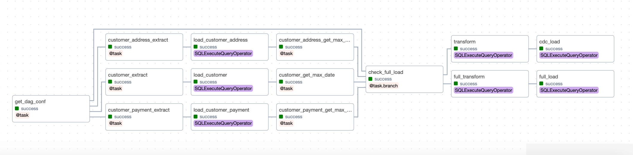
I have added two examples of the same DAG, one without custom operators and one with custom operators. You can compare, how using custom operators makes our DAG more readable and manageable, and also allows us to reuse the code across teams. Read more about Custom Operators and DAG writing best practices.
Few observations about our data pipeline
- We have created one pipeline for a business entity
customerwhich also ingests the data. But you can choose to have separate ingestion and transformation pipelines and link them using any of the methods described in Cross-DAG dependencies. - You could also use SqlToS3Operator to directly pull the data from Postgres to S3, instead of custom code and use CopyFromExternalStageToSnowflakeOperator to stage the data from S3 to Snowflake. I prefer to keep my SQL as-is because it helps in debugging.
- Even though we used an Airflow variable to store the last watermark, it is recommended to store the last watermark value in an audit table within your target database. This can help in debugging and reporting about your DAG runs.
- Our CDC process relies on the assumption that the column
updated_atis updated for each transaction in your source table allowing us to do incremental loads. - Using the same DAG for
fullanddeltaloads might not always work, depending on the amount of data that you need to process or the other operational steps required. This could result in a complex DAG which could interfere with your regulardeltaruns. Hence, you might choose to have separate DAGs for handlingfullloads. - You can also choose to use S3 as the custom XComBackend and pass the data via XCom. Then, split the
extractprocess to just pull the data from Postgres pass it to XComBackend which will directly load it to S3. Then, add another task for staging the data to Snowflake using SQLExecuteQueryOperator to allow more atomic tasks. - In our example we have relied on the same reusable path for each file in cloud storage. However, it is recommended to use Airflow DAG’s logical date as part of the file path, allowing us to keep history of the files. For example, we can set the following nomenclature for the file paths:
s3://mk-edu/incoming/pg_data/<YYYYMMDD>/customer/<customer_delta_YYYYMMDDHHMMSS>.csvThis is also helpful in re-processing DAG Runs in case of source data issues. But backfills in CDC are tricky and would require manual intervention and data correction depending on the data to be corrected and the window of correction.
- We have not handled
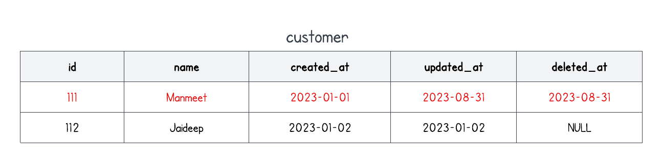
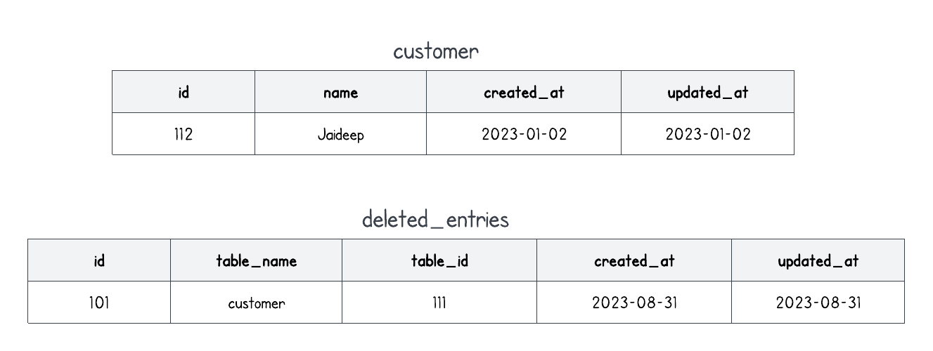
DELETEtransactions in our pipeline. To handle these, we need to understand how the source system records these transactions - soft-delete or hard-delete. Soft-delete is a process in which the record is actually not deleted from the table, but marked as deleted using a separate column likedeleted_at. This column will hold the deletion timestamp for the deleted records and will be null otherwise. Hard-delete is a process in which the record to be deleted is first inserted into a separate table and then deleted from the main table. For example:- Soft-delete
- Hard-delete
The queries to process data will change accordingly, checkout the examples in the GitHub repo for soft-delete and hard-delete.Since we are using Snowflake as an example, it is important to note that, even though Snowflake Time Travel provides access to historical data, it is only available within a defined period. It cannot be considered a replacement for CDC. Snowflake Streams provide the metadata about the changes, but you would still need to ingest the data into your external stage or a table in Snowflake and then write queries to perform CDC using Airflow.
Schema evolution
Imagine in our sample app, we also want to record the date-of-birth of a customer. This means a new column needs to be added to the source table and which needs to be propagated to our DWH. This is a common use case, especially in the early development stages of your application. To handle this in our data pipeline, we can have a task which before staging the data to Snowflake, will compare the source and target table’s structures and apply new columns identified. For example, we can add a new task before staging the data in Snowflake, which will perform the following steps:
def schema_evolution(source_table: str):
    import pandas as pd

  ## Get the columns in source
    pg_hook = PostgresHook(
        schema='postgres',
        postgres_conn_id='postgres',
    )
    with pg_hook.get_conn() as pg_conn:
     source_sql = f"""
         select lower(column_name) as \"column_name\"
         from information_schema.columns
         where table_schema = 'public'
         and table_name = '{source_table}'
     """
     source_df = pd.read_sql(source_sql, pg_conn).sort_values(by=['column_name'])
     print(source_df)

  ## Get the columns in target
    sf_hook = SnowflakeHook(
        snowflake_conn_id='snowflake'
    )
    with sf_hook.get_conn() as sf_conn:
     target_table = f'{source_table}'.upper()
     target_sql = f"""
         select lower(column_name) as \"column_name\"
         from information_schema.columns
         where table_schema = 'STAGE'
         and table_name = '{target_table}'
     """
     target_df = pd.read_sql(target_sql, sf_conn).sort_values(by=['column_name'])

  ## find the new columns
    source_cols = source_df['column_name'].tolist()
    target_cols = target_df['column_name'].tolist()
    missing_cols = list(set(source_cols) - set(target_cols))

    print("Found missing cols: ", missing_cols)
  sql_list = []
    for col in missing_cols:
        sql_list.append(f"alter table stage.{target_table} add column {col} string")
    return
Please note that the front-end team might decide to drop some columns as well. Typically, we do not drop columns from DWH or target tables, because we want to keep the history and do not want to lose the data we have already captured. This also brings us to an important point, to never use * in your SQL queries and always use explicit column names. (This is also important for your SQL’s performance in columnar databases).
Ingest directly from cloud storage
In our data pipeline, we have used pull-based approach to retrieve the data from the source database directly. Many organizations rely on a push-based approach, in which the files are sent to their SFTP server or a cloud storage. During an initial push, a full file is sent and subsequently, delta files are sent. When we rely on an external system for sending us the data, it is best to have a sensor task that will trigger the downstream pipeline to process the data. This will make our DAG event-driven and ensure that it will not fail due to minor delays in receiving the file.
Hence, in our current data pipeline, we can replace the extract task with a sensor task, S3KeySensorAsync. For example:
from astronomer.providers.amazon.aws.sensors.s3 import S3KeySensorAsync
check_for_file = S3KeySensorAsync(
  poke_interval=60,
  timeout=600,
  bucket_key='pgdata/customer',
  bucket_name='mk-edu',
  check_fn=MY_CHECK_FN,
  aws_conn_id='aws',
  deferrable=True
)
Read more about Deferrable operators and Sensor best practices.
With the custom configuration of the incoming file paths, we can rely on Airflow’s REST API to clear the DAG Runs that need to be re-run, which can then re-process the files based on the correct logical date.
Log-based sync and ELT
Up until now, we have discussed scenarios where the data sync between the source and the target system is a batch process. Now, let’s consider an ELT setup where the data from our app needs to be replicated in near-real-time to our Data Lake. To achieve this, we have a couple of options, for example:
- Choose to setup our own logical decoding for Postgres
- Setup Debezium to capture the changes from our source database
Except for the first one, the other three options require you to write a custom CDC process to sync the target schema with the source data.
The concept of logical replication is based on Write Ahead Logs, which captures the type of transaction,
DELETE,INSERT, orUPDATE, transaction metadata, and a BEFORE and AFTER image of the record. This generates a complete audit trail of changes to your database.
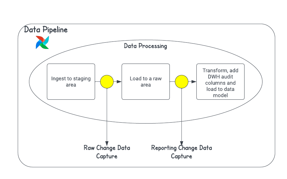
As you can observe, we might end-up having two CDC processes in our data pipeline! The first CDC process after ingestion typically updates the raw table directly without maintaining any row-wise history. This is a common pattern in an EL data pipeline. Many organizations might do away with the second CDC and rebuild the entire reporting tables everyday or follow Lambda architecture.
Lambda architecture is a hybrid approach of batch-based CDC and real-time CDC. It is especially useful in cases when the volume of data is very high. This approach aims to achieve the balance of batch-based and low-latency of real-time loads.
You might choose to rebuild some of your reporting tables when you are in the infancy phase of reporting, or your target database has no or limited ACID support. In such cases, you can implement a transformation-only pipeline to create-and-replace your target table or materialized view, or append to your target table. For example, once the raw data in your data lake is brought in sync with your source system using an EL pipeline, you can re-generate the reporting tables using a batch process and swap out the tables (or just individual partitions in a table). Log-based sync deserves its own in-depth blog!
What do you think about creating an EL pipeline that handles ingestion from log-based sync? This can be a cool addition etl-airflow GitHub repo. Feel free to contribute!
Conclusion
Change Data Capture is a vast topic which can be handled in various different ways based on your business requirements and also the personal preference of your Solutions Architect. Irrespective of the implementation of your CDC process, we must keep in mind the following when designing the data pipelines:
- Business requirement for the sync, batch - inter-day or intra-day - or real-time. This will also help you decide the type of tools you choose along with Airflow. See Schedule DAGs in Airflow.
- The ability to handle
fullvsincrementalloads. You can choose to have a separate DAG or the same DAG can be repurposed. See DAG params. - The amount of data to be processed. If you pass a lot of data between tasks, remember to always use a custom XComBackend.
- The ability to restart or rerun your pipelines in case of any failures. Modularity and atomicity of your tasks can help you effectively achieve this. See Rerun Airflow DAGs and tasks.
- Due to the variety of data we process today, the structure of the data - structured, semi-structured or unstructured - is also an important factor to consider. An EL & T pipeline is best suited for semi-structured or unstructured data. This is an interesting topic for another blog!
Try out Airflow on Astro for free and build your own data pipelines using our Learn guides.

Get started free.
OR
By proceeding you agree to our Privacy Policy, our Website Terms and to receive emails from Astronomer.