ELT with Apache Airflow® and Databricks

Overview

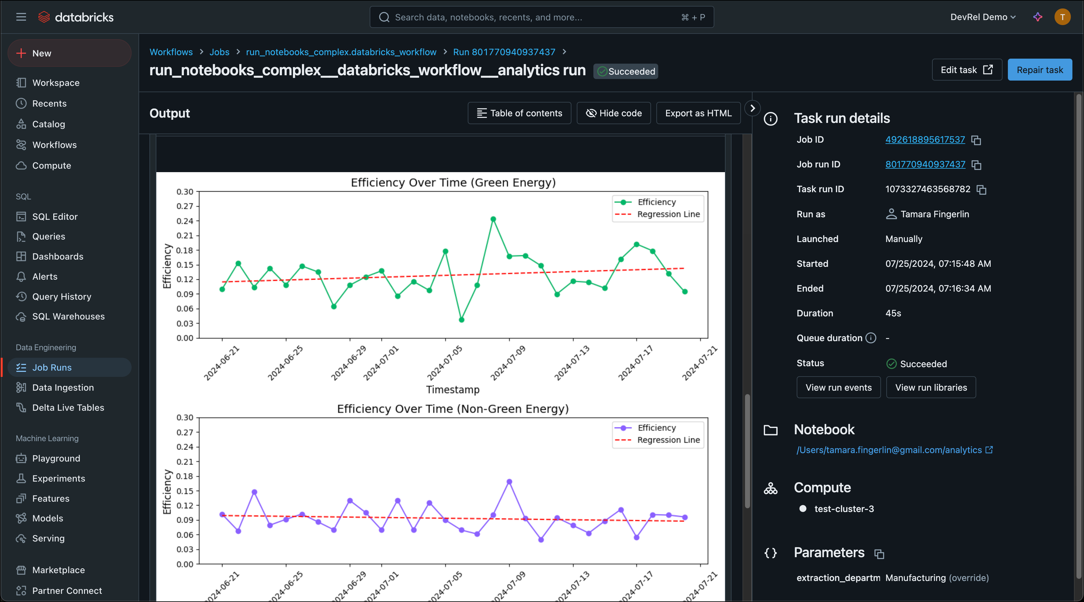
This reference architecture shows how to use Apache Airflow® to copy synthetic data about a green energy initiative from an S3 bucket into a Databricks table and run several Databricks notebooks as a Databricks job to analyze the data. A demo of the architecture is shown in the How to Orchestrate Databricks Jobs Using Airflow webinar.

Databricks is a unified data and analytics platform built around fully managed Apache Spark clusters. Using the Airflow Databricks provider package, you can create a Databricks job from Databricks notebooks running as a task group in your Airflow Dag. This lets you use Airflow’s orchestration features in combination with Databricks Workflows, Databricks’ most cost-effective compute option. For detailed instructions on using the Airflow Databricks provider, see Orchestrate Databricks jobs with Airflow.

You can adapt this architecture for your use case by changing the data source, adjusting the notebook logic, or adding transformation steps.

Architecture

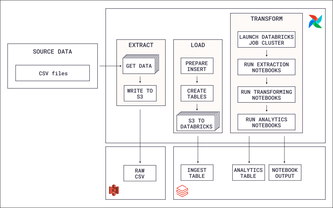
This reference architecture consists of three main components:

• Extraction: An Airflow Dag moves CSV files containing green energy data from the local filesystem to an S3 bucket using the Airflow Object Storage API.
• Loading: A second set of tasks loads the files from S3 into a Databricks table using the DatabricksCopyIntoOperator. Each file is loaded in parallel through dynamic task mapping.
• Transformation: Databricks notebooks run as a Databricks job orchestrated by Airflow using the DatabricksWorkflowTaskGroup and DatabricksNotebookOperator. The notebooks extract data from the table, transform it, and load the results back into Databricks tables.

Data flows in a clear sequence: local CSV files to S3 to a Databricks raw table to transformed tables via notebooks. The first Dag handles extraction and loading, then publishes an asset that triggers the second Dag for transformation.

Airflow features

• Airflow Databricks provider: The Databricks provider package creates Databricks jobs directly from Airflow. The DatabricksWorkflowTaskGroup wraps multiple notebooks into a single Databricks Workflow job, while operators like DatabricksSqlOperator and DatabricksCopyIntoOperator handle SQL execution and data loading.
• Task groups: The Databricks notebook execution is wrapped in a task group that maps to a single Databricks Workflow job. This keeps the Dag graph readable and allows the group to be collapsed in the Airflow UI.
• Dynamic task mapping: Loading data from S3 into Databricks is parallelized per file using dynamic task mapping. The number of files is determined at runtime, so the Dag adapts automatically when new files are added to the S3 bucket.
• Object Storage: The Airflow Object Storage API simplifies moving files to S3 without writing provider-specific code. Files are streamed between paths, which keeps memory usage low even for large datasets.
• Data-aware scheduling: The extraction and loading Dag runs on a time-based schedule and publishes an asset when loading completes. The transformation Dag schedules itself on this asset, so it only triggers when fresh data is available in Databricks.

Next steps

To build your own ELT pipeline with Databricks and Apache Airflow, explore the individual Learn guides linked in the Airflow features section for detailed implementation guidance on each pattern. Astronomer recommends deploying Airflow pipelines using a free trial of Astro.