Snowflake Anomaly Detection with SnowPatrol

Introducing SnowPatrol

SnowPatrol is an application for anomaly detection and alerting of Snowflake usage powered by Machine Learning. It’s
also an MLOps reference implementation, an example of how to use Airflow as a way to manage the training, testing,
deployment, and monitoring of predictive models.

In this three-part blog post series, we’ll explore how we built SnowPatrol to help us proactively identify abnormal
Snowflake usage (and cost) and simplify overage root-cause analysis and remediation.

Part 1 lays the foundation of our solution. We detail our motivations and dive into how Snowflake pricing works. We also
take a closer look at the available data, and how an isolation forest model can be used to detect unexpected cost
overages.

Part 2 covers how Astro customers (including Astronomer’s own data team) have used these methods to convert detected
anomalies into actionable insights. We introduce a handy anomaly exploration plug-in that enhances SnowPatrol’s
capabilities. We also explore how anomalies can be used to track down problematic DAGs and remediate issues.

Finally, in Part 3, we’ll discuss the optimization of SnowPatrol, covering topics such as model monitoring,
champion-challenger deployment, and the exploration of new model architectures to further improve the tool’s performance
and effectiveness.

Get ready to learn how SnowPatrol can help you tackle your cloud costs head-on!

At Astronomer, we firmly believe in the power of open source and sharing knowledge. We are excited to share this MLOps
reference implementation with the community and hope it will be useful to others. All the code and documentation is
available on GitHub. You can find it here.

Why Snowflake Anomaly Detection Matters

Astronomer is a data-driven company, and we rely heavily on Snowflake to store and analyze our data. Self-service
analytics is a core part of our culture, and we encourage our teams to answer questions with data themselves, either by
running SQL queries or building their own data visualizations. As such, a large number of users and service accounts run
queries on a daily basis; on average more than 900k queries are run daily. The majority of these queries come from
automated Airflow DAGs running on various schedules. Identifying which automated process or which user ran a query
causing increased usage on a given day is time-consuming when done manually. We would rather not waste
time chasing cars.

Cost management is also a key part of our operations. Just like most organizations, we want to avoid overages and
control our Snowflake costs. While that is a common goal, it can be challenging to achieve. Snowflake costs are complex
and can be attributed to a variety of factors.

Increased storage costs can be attributed to growing tables, staged files for bulk data loading, fail-safe data
retention for time travel and clones and more.

Increased compute costs can come from different sources: virtual warehouses used to run queries, serverless features
used for maintenance & automation, as well as cloud services. Additionally, the natural growth of data pipelines can go
unnoticed. This growth can catch teams off guard, especially when it exceeds what was initially anticipated during the
annual planning phase with Snowflake. The unpredictability of annual usage underscores the importance of proactive
monitoring and adaptation to evolving data needs.

Through exploratory data analysis, we learned early on that 99% of our Snowflake costs come from virtual warehouse
computing. With that information in hand, we chose not to look at storage cost in the first version and focused solely
on identifying abnormal daily usage for virtual warehouses. Future work will be done to address storage costs as well.
At its core, our solution aims to be very simple. When higher than normal usage is detected, we notify admins and
provide them with the necessary information to assist in root cause analysis.

In practice, attributing Snowflake costs back to the specific DAG and Task that ran queries is not always trivial. Query
Tags can be used to accomplish this, but it requires that every query be tagged appropriately. We will discuss how this
can be automated with SnowPatrol in Part 2.

How Snowflake Pricing Works

Snowflake pricing tiers depend on variables such as the cloud provider, region, plan type, services, and more. Snowflake
costs are grouped into two distinct categories: storage and compute.

Storage: Storage is calculated monthly based on the average number of on-disk bytes stored each day.
Compute: Compute costs represent credits used for:

• The number of virtual warehouses you use, how long they run, and their size.
• Cloud services that coordinate activities across Snowflake, such as authentication, infrastructure management, query
  parsing and optimization, and access control.
• Serverless features such as Snowpipe, Snowpipe streaming, Database Replication, Materialized Views, Automatic
  Clustering and Search Optimization

For all the details, you can read Snowflake’s documentation here:
https://docs.snowflake.com/en/user-guide/cost-understanding-overall
and here https://www.snowflake.com/pricing/pricing-guide/

Uncovering Patterns in Snowflake Usage Data

Notebooks play a crucial role in exploring and understanding the data used to train the isolation forest model. By
leveraging Jupyter Notebook’s interactive environment, we can easily load and manipulate the relevant datasets using
libraries like snowflake-connector and pandas. This allows us to move fast to gain insights into the data’s structure
and get rapid feedback as we iteratively perform the necessary preprocessing steps.

Jupyter Notebook’s ability to visualize data using libraries such as Matplotlib and Seaborn helps in identifying
patterns, outliers, and anomalies visually, which is essential for understanding the business problem we are working to
solve.

Moreover, the Jupyter Notebook enables us to experiment with different feature engineering techniques and test the
isolation forest model’s performance. This iterative process of data exploration and model refinement is crucial in
developing a robust and effective anomaly detection system like SnowPatrol.

Snowflake usage and metering information can be fetched from the USAGE_IN_CURRENCY_DAILY
and WAREHOUSE_METERING_HISTORY views in the ORGANIZATION_USAGE schema.

Using the data from those two tables we can better understand what costs us money and build the right solution to
address it.

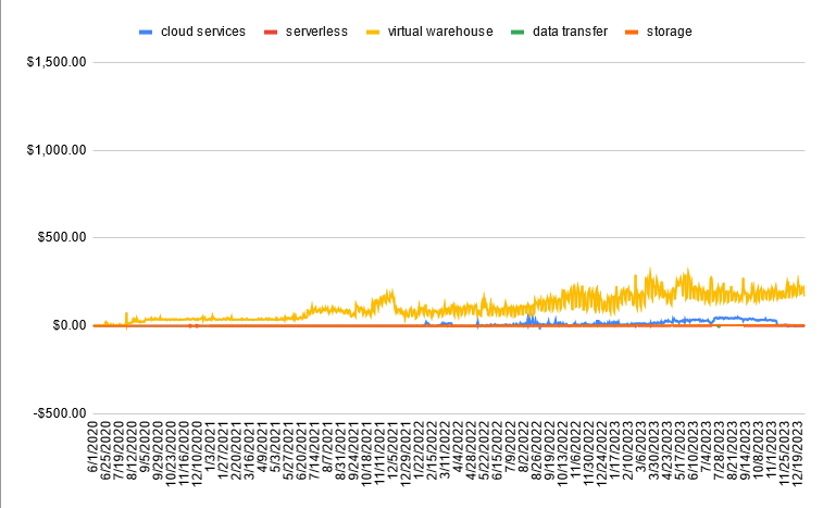
Looking at the usage by cost category, we find virtual warehouses and cloud services are the biggest expenses. We can
also start to see cyclical patterns at a high level.

Knowing that Virtual Warehouses are our biggest cost category we can focus our attention on it and dive deeper. Let’s
break it down by Warehouse to see how costs fluctuated over the last year.

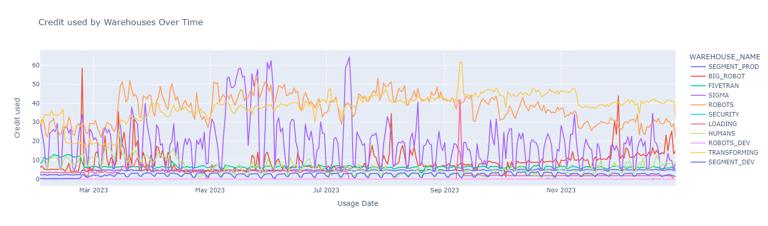
Diving deeper and looking at individual warehouses, we can confirm Warehouse costs follow cycles and anomalies are
present.

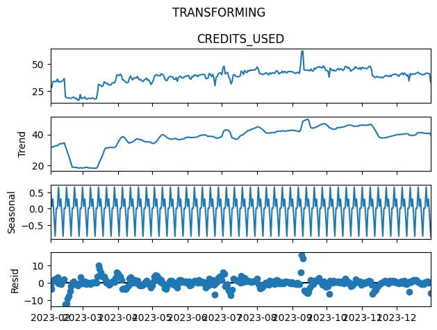
Next, we will look at how we can, for individual warehouses, extract seasonal cycles and trends and focus our attention
on outliers. By decomposing the time series, we can isolate seasonality and trend and outliers will show up in the
residuals.

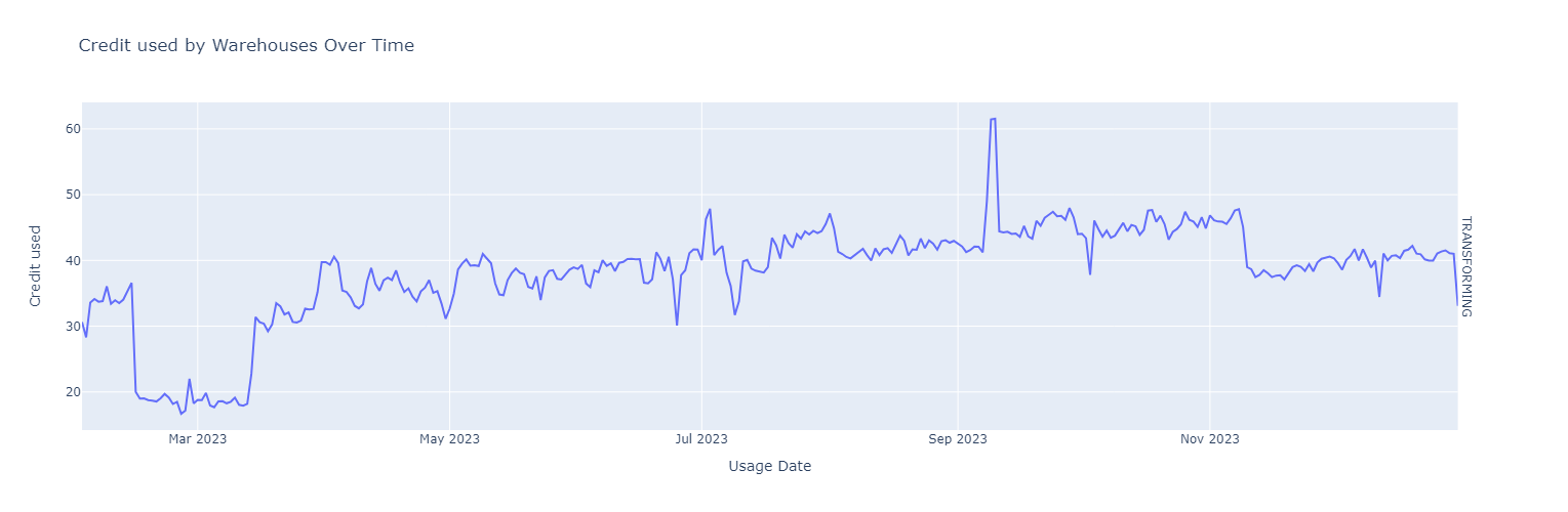
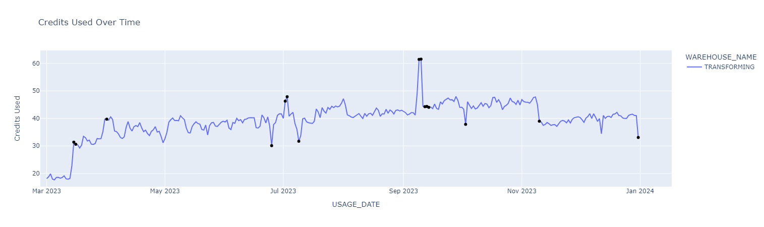
We use STL decomposition for simplicity. STL is an acronym for “Seasonal and Trend decomposition using Loess”. This
technique gives you the ability to split your time series signal into three parts: seasonal, trend, and residue. It
works well for time series with recurring patterns such as periodically repeating DAGs with predefined schedules.
Here is what it looks like for a single warehouse before we perform the decomposition.

And here is what it looks like after the decomposition. We can see the trend, seasonality and residuals. Anomalies are
visible in the residuals in the bottom chart.

Pinpointing Anomalies in Snowflake Usage with Machine Learning

Now that we have decomposed our Warehouse cost time series and extracted trends and seasonality, we use an unsupervised
approach with an Isolation Forest model to detect anomalies in the residuals.

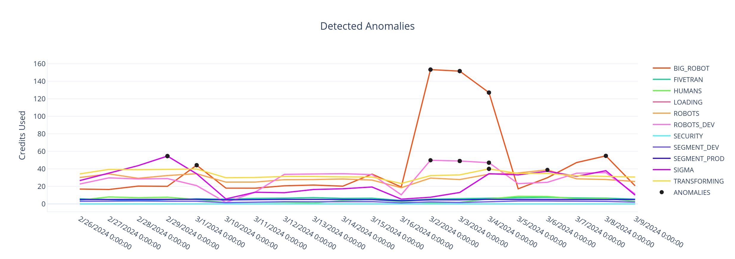
We use an anomaly threshold of 2 standard deviations from the mean of the stationary decomposed residual data to detect
anomalies. Any value outside of this threshold is flagged as an anomaly. Once we plot the abnormal values back on top of
the credit usage time series, here is what it looks like.

Separate models are trained for each warehouse since each is used for different use cases and has different consumption
patterns.

Automating Anomaly Detection: The Power of Airflow and Machine Learning

Airflow is the tool of choice for building high-impact data solutions. In SnowPatrol, we leverage it for the
orchestration of both data transformation and machine learning workflows: data preparation, feature engineering, model
training, anomaly detection, reporting and alerting. Airflow’s scalability and flexibility allow it to handle complex
pipelines with thousands of tasks, while its modular architecture enables easy customization and extensibility to fit
the specific needs of our project. The ability to dynamically generate pipelines using Python code empowers us to create
sophisticated workflows that adapt based on input parameters and conditionally execute tasks.

Airflow’s rich ecosystem of ready-made operators and hooks allows for simple integrations with external systems. In
SnowPatrol, this allows us to easily interact with Snowflake and Weights & Biases. Additionally, Airflow provides
powerful scheduling capabilities, enabling us to define the frequency and dependencies of our tasks, as well as support
backfilling to rerun past workflows or catch up on missed runs, ensuring data consistency and completeness.

Moreover, the simple UI lets us quickly see what was executed each time the data was prepared and the model was
retrained. Airflow’s ability to retry failed tasks, monitor pipeline logs, and trigger alerts ensures the reliability
and robustness of our pipelines. The platform also allows us to define the level of parallelism for our tasks,
optimizing the performance of our pipelines based on available infrastructure.

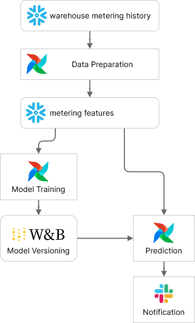
Here is a simple flow diagram illustrating SnowPatrol’s Airflow DAGs. We will dive deeper into each one, but first,
let’s explore the different Airflow features used to orchestrate SnowPatrol.

Key Airflow Features for Efficient Anomaly Detection

The workflow management capabilities listed above apply well to ML workloads in general. To develop this particular
solution we leveraged several additional Airflow features. Let’s dive into the two most important ones and see how they
help us achieve our goals.

Data-Aware Scheduling

Astronomer recommends using Airflow’s data-aware scheduling when your pipeline tasks depend on the availability or
freshness of specific datasets.

Data-aware scheduling allows you to define dependencies between tasks based on the presence or modification time of
datasets, ensuring that downstream tasks only execute when the required data is ready. This feature helps optimize
resource utilization, reduce unnecessary computations, and ensure that your tasks are executed in the correct order
based on data dependencies.

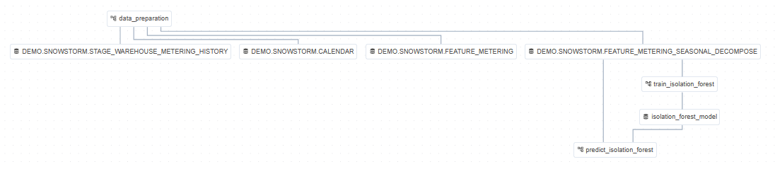
In SnowPatrol, our data preparation DAG is configured to run daily. We use data-aware scheduling to trigger downstream
DAGs once the Data Preparation is complete and data is made available. This allows us to trigger the Model Training DAG
once the feature dataset is available in Snowflake. Our prediction DAG fires after both Data Preparation and Model
Training are complete ensuring we always use the latest data and the most recent model to detect anomalies.
Airflow also allows us to visualize the dependencies between datasets in the UI. Here is what it looks like

Dynamic Task Mapping

Astronomer recommends using Airflow’s dynamic task mapping when your pipeline needs to dynamically generate tasks based
on input data or parameters. Dynamic task mapping allows you to create a set of tasks at runtime, enabling your pipeline
to adapt to changing requirements or scale according to the input data. It applies particularly well to training models
in parallel, say for hyperparameter optimization or training on different dimensions of a dataset.

In SnowPatrol we use Dynamic Task Mapping to train multiple models according to the list of existing Snowflake
Warehouses. The full list is determined at runtime by querying Snowflake and may change over time.

How SnowPatrol Detects Anomalies: The DAG breakdown

Data preparation, model training, and anomaly detection are managed through distinct workflows. By creating individual
Airflow DAGs for each of these workflows, they can be scheduled independently. Despite their independence, these
workflows are interconnected. We use Airflow’s Data-aware Scheduling with Datasets to define dependencies between the
DAGs and coordinate their execution.

Data Preparation

Snowflake performs nightly updates to the metering statistics and makes the data available in
the WAREHOUSE_METERING_HISTORY table. While we could use the tables directly, the data is truncated daily and only the
last 365 days are kept.

The data preparation DAG extracts organization-level metering data, cleans it up and accumulates it so we have a full
history. To keep things simple, data validation and feature engineering are done as part of the same DAG.

Validation

A task is configured to perform data validation of the raw data to ensure it has been loaded for all past dates. If any
dates are missing, our team is alerted and we can investigate the ingestion issue.

Feature Engineering

Metering data is transformed for each warehouse. We decompose the seasonality of the metering data into trend, seasonal,
and residual components, then persist the data in Snowflake.

Model Training

Multiple models are trained and versioned in the model catalog. Downstream inference tasks use the latest model
available to detect anomalies. The Isolation Forest model training DAG is triggered when data drift is detected in the
metering data. Dynamic task mapping is used to train models for each warehouse.

Tracking Models and Experiments

This project uses Weights and Biases for experiment and model tracking. We use
the DAG run_id of the model training DAG to group all model instances. This way we can easily see the models trained for
each warehouse in the same run. Each model has an anomaly_threshold parameter which is threshold_cutoff (default is 2)
standard deviations from the mean of the stationary (decomposed residual) scored data. Additionally, artifacts are
captured to visualize the seasonal decomposition and the anomaly scores of the training data. These are logged to the
Weights and Biases project along with the model and anomaly_threshold metric.

Model Versioning

Successful runs of the training DAG tag models are marked as “latest” in
the Model Registry. The downstream anomaly detection DAG can then use this tag to
download the appropriate model and detect anomalies. Future work will include champion/challenger model promotion based
on model performance metrics.

Predictions and Alerting

Predictions are made in batches with dynamic tasks for each model instance. Identified anomalies are grouped and a
report is generated in Markdown format. Alerts are sent as Slack messages for notification. An Airflow Plugin is also
available to explore the anomalies. In a future version, the plugin will allow users to label anomalies to allow for
supervised learning models to be trained.

Stay tuned for Part 2 of this blog series where we dive into how to make use of the detected anomalies to cut costs.

Next Steps

Part 2 will cover how we at Astronomer convert detected anomalies into actionable insights. We introduce a handy anomaly
exploration plugin that enhances SnowPatrol’s capabilities. We will also explore how anomalies can be used to track down
problematic DAGs and remediate issues.

Thanks to a collaboration with the Data engineering team at Grindr, we will also explore how Snowflake Query Tags can be
used to link expensive queries to Airflow Tasks. This allows us to know exactly how much each DAG costs to run.
In Part 3, we’ll discuss the optimization of SnowPatrol, covering topics such as model monitoring, champion-challenger
deployment, and the exploration of new model architectures to further improve the tool’s performance and effectiveness.
A/B testing of models will be added to the model training DAG. We will use the Weights and Biases API to track model
performance and compare models.

Other model architectures will be explored. We will try to use additional model features to detect anomalies over
multiple days. We will also explore the use of supervised learning models once our database of labelled anomalies is
large enough.

Conclusion

SnowPatrol is a simple yet powerful application for anomaly detection and alerting of Snowflake usage powered by Machine
Learning and Airflow. With it, we can react swiftly to abnormal usage, improve our data engineering practices, avoid
overages and reduce our Snowflake costs.

We are excited to share this project with the community and hope it will be useful to others. We are looking forward to
your feedback and contributions.

Give us your feedback, comments and ideas at https://github.com/astronomer/snowpatrol/discussions