Use setup and teardown tasks in Airflow
Info
This page has not yet been updated for Airflow 3. The concepts shown are relevant, but some code may need to be updated. If you run any examples, take care to update import statements and watch for any other breaking changes.
In production Airflow environments, it’s best practice to set up resources and configurations before certain tasks can run, then tear the resources down even if the tasks fail. This pattern can reduce resource utilization and save costs.
Starting in Airflow 2.7, you can use a special type of task to create and delete resources. In this guide, you will learn all about setup and teardown tasks in Airflow.

Other ways to learn
There are multiple resources for learning about this topic. See also:
- Webinar: What’s New in Airflow 2.7.
- Webinar: Efficient data quality checks with Airflow 2.7.
Assumed knowledge
To get the most out of this guide, you should have an understanding of:
- Airflow decorators. See Introduction to the TaskFlow API and Airflow decorators.
- Managing dependencies in Airflow. See Manage task and task group dependencies in Airflow.
When to use setup/ teardown tasks
Setup/ teardown tasks ensure that the necessary resources to run an Airflow task are set up before a task is executed and that those resources are torn down after the task has completed, regardless of any task failures.
Any existing Airflow task can be designated as a setup or teardown task, with special behavior and added visibility of the setup/ teardown relationship in the Airflow UI.
There are many use cases for setup and teardown tasks. For example, you might want to:
- Manage a Spark cluster to run heavy workloads.
- Manage compute resources to train an ML model.
- Manage the resources to run data quality checks.
- Set up storage in your custom XCom backend to hold data processed through Airflow tasks, then tear the extra storage down afterwards when the XCom data is no longer needed.
Setup/ teardown concepts
Any task can be designated as a setup or a teardown task. A setup task, its teardown task, and the tasks in between constitute a setup/ teardown workflow.
Tasks that run after a setup task and before the associated teardown task are considered to be in scope of the setup/ teardown workflow. Usually these tasks will use the resources set up by the setup task and which the teardown task will dismantle.
Setup/ teardown tasks have different behavior from regular tasks:
-
Clearing a task that is in scope of a setup/ teardown workflow will also clear and rerun the associated setup and teardown tasks, ensuring that all resources the task needs are created again for the task rerun and torn down after the task has completed.
-
A teardown task will run as long as at least one of its associated setup tasks have completed successfully and all of its upstream tasks have completed, regardless of whether they were successful or not. If all associated setup tasks fail or are skipped, the teardown task will be failed or skipped respectively.
-
A teardown task without any associated setup tasks will always run once all upstream worker tasks have completed running, independently of whether they were successful or not.
-
When evaluating whether a DAG run was successful, Airflow will ignore teardown tasks by default. This means if a teardown task fails as the final task of a DAG, the DAG is still marked as having succeeded. In the example shown in the screenshot below, the DAG run state is not impacted by the failure of
tear_down_clusterand is marked as successful. You can change this behavior by settingon_failure_fail_dagrun=Truein the.as_teardown()method or@teardowndecorator.
-
When a teardown task is within a task group and a dependency is set on the task group, the teardown task will be ignored when evaluating if a dependency has been met. For example,
run_after_task_group, which is dependent on thework_in_the_clustertask group, will run even if the teardown task has failed or is still running.
-
You can have a setup task without an associated teardown task and vice versa. If you define a setup task without a teardown task, everything downstream of the setup task is considered in its scope and will cause the setup task to rerun when cleared.
Before and after using setup and teardown tasks
Setup and teardown tasks can help you write more robust DAGs by making sure resources are set up at the right moment and torn down even when worker tasks fail.
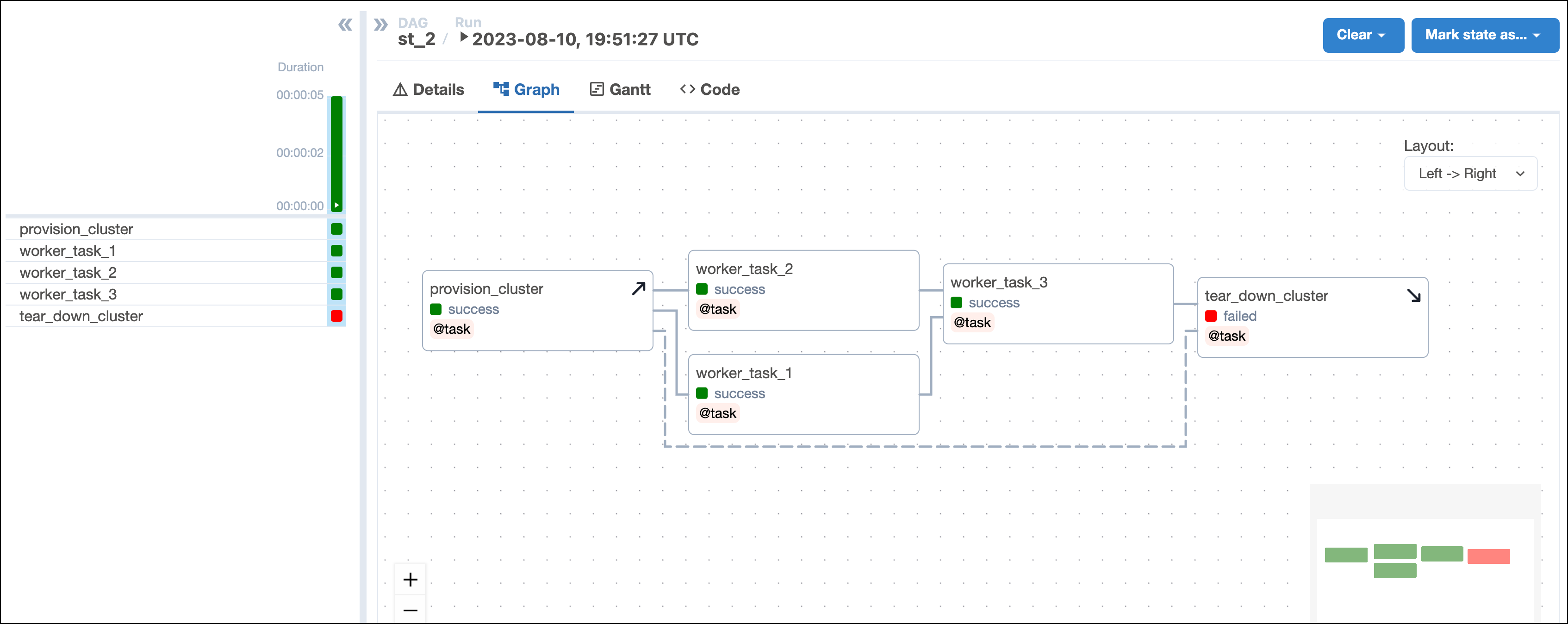
The following DAG is not using Airflow setup and teardown functionality. It sets up its resources using a standard task called provision_cluster, runs three worker tasks using those resources, and tears down the resources using the tear_down_cluster task.

The way this DAG is set up, a failure in any of the worker tasks will lead to the tear_down_cluster task not running. This means that the resources will not be torn down and will continue to incur costs. Additionally, any downstream tasks depending on tear_down_cluster will also fail to run unless they have trigger rules to run independently of upstream failures.

In this example, you can turn the provision_cluster task into a setup task and the tear_down_cluster into a teardown task by using the code examples shown in setup/ teardown implementation.
After you convert the tasks, the Grid view shows your setup tasks with an upwards arrow and teardown tasks with a downwards arrow. After you configure the setup/ teardown workflow between provision_cluster and tear_down_cluster, the tasks are connected by a dotted line. The tasks worker_task_1, worker_task_2 and worker_task_3 are in the scope of this setup/ teardown workflow.

Now, even if one of the worker tasks fails, like worker_task_2 in the following screenshot, the tear_down_cluster task will still run, the resources will be torn down, and downstream tasks will run successfully.

Additionally, when you clear any of the worker tasks, both the setup and teardown tasks will also be cleared and rerun. This is useful when you are recovering from a pipeline issue and need to rerun one or more tasks that use a resource independent of the other tasks in the scope.
For example, in the previous DAG, consider if worker_task_2 failed and worker_task_3 was unable to run due to its upstream task having failed. If you cleared worker_task_2 by clicking Clear task, both the setup task provision_cluster and the teardown task tear_down_cluster will be cleared and rerun in addition to worker_task_2, worker_task_3 and downstream_task. This lets you completely recover without needing to rerun worker_task_1 or manually rerun individual tasks.

Setup/ teardown implementation
There are two ways to turn tasks into setup/ teardown tasks:
- Using the
.as_setup()and.as_teardown()methods on TaskFlow API tasks or traditional operators. - Using the
@setupand@teardowndecorators on a Python function.
Worker tasks can be added to the scope of a setup/ teardown workflow in two ways:
- By being between the setup and teardown tasks in the DAG dependency relationship.
- By using a context manager with the
.teardown()method.
Which method you choose to add worker tasks to a setup/ teardown scope is a matter of personal preference.
You can define as many setup and teardown tasks in one DAG as you need. In order for Airflow to understand which setup and teardown tasks belong together, you need to create setup/ teardown workflows.
.as_setup() and .as_teardown() methods
Any individual task can be turned into a setup or teardown task.
To turn a task into a setup task, call the .as_setup() method on the called task object.
Taskflow

Traditional

To turn a task into a teardown task, call the .as_teardown() method on the called task object. Note that you cannot have a teardown task without at least one upstream worker task.
Taskflow

Traditional

After you have defined your setup and teardown tasks you need to define their workflow in order for Airflow to know which setup and teardown tasks perform actions on the same resources.
@setup and @teardown decorators
When working with the TaskFlow API you can also use the @setup and @teardown decorators to turn any Python function into a setup or teardown task.

As with the .as_teardown() method you cannot have a @teardown task without at least one upstream worker task. The worker task can use the @task decorator or be defined with a traditional operator.

After you have defined your setup and teardown tasks you need to create their workflows in order for Airflow to know which setup and teardown tasks perform actions on the same resources.
Creating setup/ teardown workflows
Airflow needs to know which setup and teardown tasks are related based on the resources they manage. Setup and teardown tasks can be defined in the same workflow by:
- Providing the setup task object to the
setupsargument in the.as_teardown()method of a teardown task object. - Connecting a setup and a teardown task with a normal task dependency using the bit-shift operator (
>>) or a dependency function likechain(). - Providing the called object of a task created using the
@setupdecorator as an argument to a task created using the@teardowndecorator.
Which method you use is a matter of personal preference. However, note that if you are using @setup and @teardown decorators, you cannot use the setups argument.
You can have multiple sets of setup and teardown tasks in a DAG, both in parallel and nested workflows.
There are no limits to how many setup and teardown tasks you can have, nor are there limits to how many worker tasks you can include in their scope.
For example, you could have one task that creates a cluster, a second task that modifies the environment within that cluster, and a third task that tears down the cluster. In this case you could define the first two tasks as setup tasks and the last one as a teardown task, all belonging to the same resource. In a second step, you could add 10 tasks performing actions on that cluster to the scope of the setup/ teardown workflow.
There are multiple methods for linking setup and teardown tasks.
Taskflow_Setups
Using the @task decorator, you can use the .as_teardown() method and the setups argument to define which setup tasks are in the same workflow as the teardown task. Note that it is also possible to use @setup and @teardown decorators instead and link them using direct dependencies.

Traditional_Setups
If you are using traditional Airflow operators, you can use the .as_teardown() method and the setups argument to define which setup tasks are in the same workflow as the teardown task.

Taskflow_Direct
Instead of using the setups argument you can directly link the setup and teardown tasks with a traditional dependency. Whenever you define a direct dependency between a setup and a teardown task Airflow will interpret this as them being in the same workflow together, no matter what actions the tasks actually perform.
This code creates an identical DAG using the setups argument.

Decorators
With the@setup and @teardown decorators, you can define the setup/ teardown workflow between two tasks either by defining direct dependencies or by providing the object of the setup task as an argument to the teardown task.
The latter pattern is often used to pass information like a resource id from the setup task to the teardown task.

Context_Manager
You can also use a task that calls the .as_teardown() method to wrap a set of tasks that should be in scope of a setup/ teardown workflow. The code snippet below shows three tasks being in scope of the setup/ teardown workflow created by my_cluster_setup_task and my_cluster_teardown_task.

Note that a task that was already instantiated outside of the context manager can still be added to the scope, but you have to do this explicitly using the .add_task() method on the context manager object.
Using multiple setup/ teardown tasks in one workflow
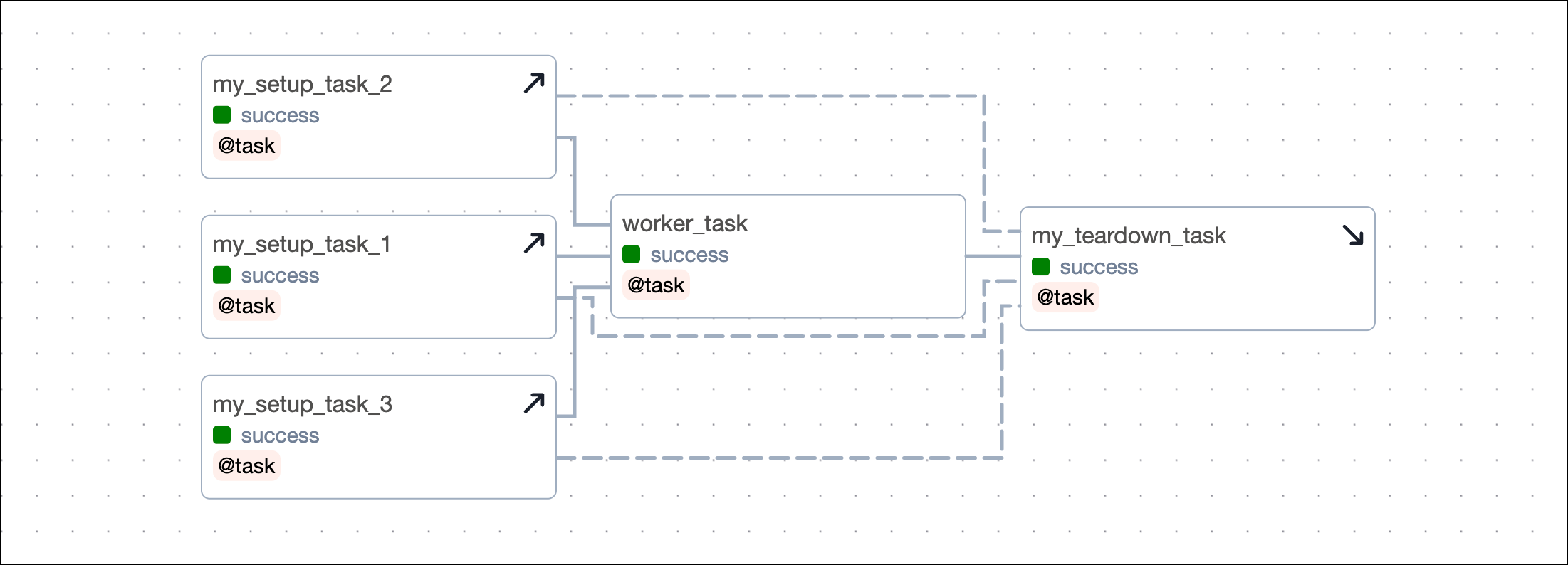
To define several setup tasks for one teardown task, you can pass a list of setup tasks to the setups argument. You do not need to call .as_setup() on any of the setup tasks.

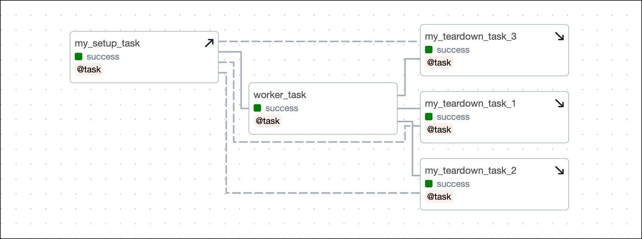
To define several teardown tasks for one setup task, you have to provide the setup task object to the setups argument of the .as_teardown() method of each teardown task.

If your setup/ teardown workflow contains more than one setup and one teardown task, you need to define several dependencies, when not using the setups argument. Each setup task needs to be set as an upstream dependency to each teardown task. The example below shows a setup/ teardown workflow containing two setup tasks and two teardown tasks. To define the workflow, you need to set four dependencies.
This code creates an identical DAG using the setups argument.

Parallel setup/ teardown workflows
You can have several independent sets of setup and teardown tasks in the same DAG. For example, you might have a workflow of tasks that sets up and tears down a cluster and another workflow that sets up and tears down a temporary database.
Decorators
Methods

Nested setup/ teardown workflows
You can nest setup and teardown tasks to have an outer and inner scope. This is useful if you have basic resources, such as a cluster that you want to set up once and then tear down after all the work is done, but you also have resources running on that cluster that you want to set up and tear down for individual groups of tasks.
The example below shows the dependency code for a simple structure with an outer and inner setup/ teardown workflow:
outer_setupandouter_teardownare the outer setup and teardown tasks.inner_setupandinner_teardownare the inner setup and teardown tasks and both are in scope of the outer setup/ teardown workflow.inner_worker_1andinner_worker_2are worker tasks that are in scope of the inner setup/ teardown workflow. All tasks in scope of the inner setup/ teardown workflow will also be in scope of the outer setup/ teardown workflow.outer_worker_1,outer_worker_2,outer_worker_3are worker tasks that are in scope of the outer setup/ teardown workflow.

Clearing a task will clear all setups and teardowns the task is in scope of, in addition to all downstream tasks. For example:
- Clearing any of the outer worker tasks (
outer_worker_1,outer_worker_2,outer_worker_3) will also clearouter_setup,outer_teardown. - Clearing any of the inner worker tasks (
inner_worker_1,inner_worker_2) will clearinner_setup,inner_teardown,outer_setup, andouter_teardown. Additionallyouter_worker_1andouter_worker_2will be cleared because they are downstream of the inner worker tasks.outer_worker_3will not be cleared because it runs parallel to the inner worker tasks.
Narrowing the scope of a setup task
If you have a setup task with no associated downstream task, you can narrow the scope of the setup task by using an empty task as its teardown. For example, if my_worker_task_3_obj does not need the resources created by my_setup_task and should not cause a rerun of the setup task when cleared, you can add an empty teardown task in the dependency chain:
Example DAG
The DAG shown in this example mimics a setup/ teardown pattern that you can run locally. The setup/ teardown workflow consists of the following tasks:
-
The
create_csvtask is a setup task that creates a CSV file in a directory specified as a DAG param. -
The
write_to_csvtask is a setup task that writes data to the CSV file. -
The
fetch_datatask is a setup task that fetches data from a remote source and writes it to the CSV file. -
The
delete_csvtask is the associated teardown task and deletes the resource of the CSV file. -
The
get_average_age_objtask is in scope of the setup/ teardown workflow. If this task fails, the DAG still needs to delete the “CSV file” afterwards (to make it more real, consider the CSV file to be an expensive cluster).To recover from a failure when rerunning the
get_average_age_objtask, you always need the CSV file to be created again, as well as the data to be fetched again and written to the CSV file. Because the task is in scope ofcreate_csv,write_to_csv, andfetch_data, these tasks will also rerun when you rerunget_average_age_obj.
The DAG contains 3 tasks which are not in scope of the setup/ teardown workflow:
- The
starttask is an empty task at the start of the DAG. - The
report_file_pathtask is a task that prints the path of the CSV file to the logs. - The
endtask is an empty task at the end of the DAG.
This DAG comes with a convenience parameter to test setup/ teardown functionality. Toggle fetch_bad_data in the Trigger DAG view to cause bad data to get into the pipeline and the get_average_age_obj to fail. You will see that delete_csv will still run and delete the CSV file. In a real-world scenario, after fixing the data issue you would clear the get_average_age_obj task and all tasks of the setup/ teardown workflow would rerun and complete successfully.
Methods
Decorators
