> ## Documentation Index
> Fetch the complete documentation index at: https://astronomer.io/docs/llms.txt
> Use this file to discover all available pages before exploring further.
# Run an integrated ELT and ML pipeline on Stripe data in Airflow
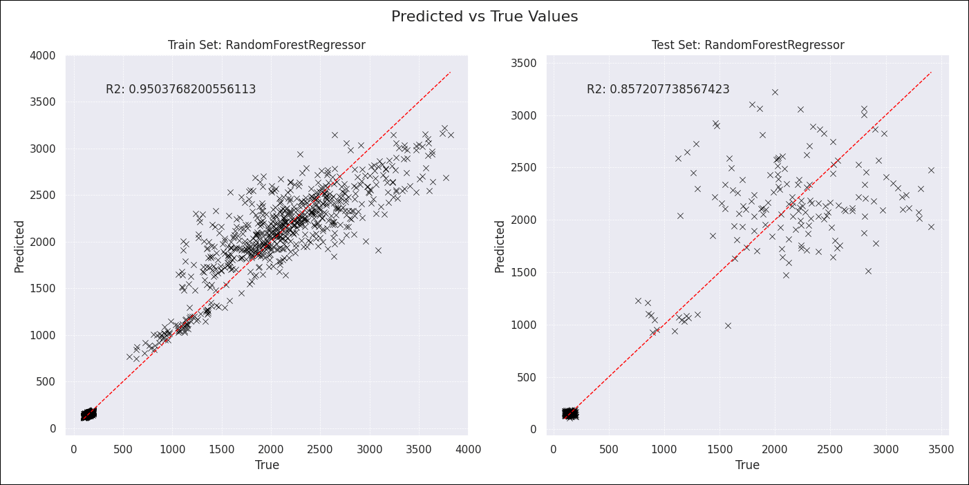
ELT/ETL and ML orchestration are two of the most common use cases for Airflow. This project shows how to use Airflow, the [Astro Python SDK](https://astro-sdk-python.readthedocs.io/en/stable/), and [Airflow Datasets](/docs/learn/2.x/airflow-datasets) to build a data-driven pipeline that combines ETL and ML. For this example, we use mock financial data modeled after the [Stripe API](https://stripe.com/docs/api/charges). Based on different customer satisfaction scores and product type we'll try to predict the total amount spent per customer, hoping to get some insight into which areas of customer satisfaction to focus on. You can adjust the model class and hyperparameters to improve model fit. What R2 can you achieve?
 ## Before you start
Before trying this example, make sure you have:
* The [Astro CLI](/docs/cli/v1.43/overview).
## Clone the project
Clone the example project from the [Astronomer GitHub](https://github.com/astronomer/use-case-elt-ml-finance). To keep your credentials secure when you deploy this project to your own git repository, make sure to create a file called `.env` with the contents of the `.env_example` file in the project root directory.
The repository is configured to spin up and use local [Postgres](https://www.postgresql.org/) and [MinIO](https://min.io/) instances without you needing to define connections or access external tools. MinIO is a local storage solution that mimics the S3 API and can be used with S3 specific Airflow operators.
If you want to use S3 as your object storage, you can change the `AIRFLOW_CONN_AWS_DEFAULT` in the `.env` file and provide your AWS credentials. To use a different relational database, [add an Airflow connection](/docs/learn/2.x/connections) to a [database supported by the Astro Python SDK](https://astro-sdk-python.readthedocs.io/en/stable/supported_databases.html) to your Airflow instance and set `DB_CONN_ID` in the DAG files to your connection ID.
## Run the project
To run the example project, open your project directory and run:
```sh wrap theme={null}
astro dev start
```
This command builds your project and spins up 6 containers on your machine to run it:
* The Airflow webserver, which runs the Airflow UI and can be accessed at `https://localhost:8080/`.
* The Airflow scheduler, which is responsible for monitoring and triggering tasks.
* The Airflow triggerer, which is an Airflow component used to run [deferrable operators](/docs/learn/2.x/deferrable-operators).
* The Airflow metadata database, which is a Postgres database that runs on port `5432`.
* A local [MinIO](https://min.io/) instance, which can be accessed at `https://localhost:9000/`.
* A local [Postgres](https://www.postgresql.org/) instance, that runs on port `5433`.
To run the project, unpause all DAGs. The `in_finance_data` and `finance_elt` DAGs will start their first runs automatically. Note that the first two tasks of the `finance_elt` DAG are deferrable operators that wait for files to be created in the object storage. The operators are set to poke once per minute, and you can change this behavior by setting their `poke_interval` to a different time span.
## Project contents
### Data source
The data in this example is generated using the [`create_mock_data`](https://github.com/astronomer/use-case-elt-ml-finance/blob/main/include/create_mock_data.py) script. The script creates CSV files in `include/mock_data` that contain data resembling the payload of the [Stripe API](https://stripe.com/docs/api/charges) Charges endpoint and customer satisfaction scores. The data is generated to contain a relationship between two features and the target variable `amount_charged`.
### Project overview
This project consists of three DAGs: one helper DAG to simulate an ingestion process and two pipeline DAGs which have a dependency relationship through [Airflow datasets](/docs/learn/2.x/airflow-datasets).
## Before you start
Before trying this example, make sure you have:
* The [Astro CLI](/docs/cli/v1.43/overview).
## Clone the project
Clone the example project from the [Astronomer GitHub](https://github.com/astronomer/use-case-elt-ml-finance). To keep your credentials secure when you deploy this project to your own git repository, make sure to create a file called `.env` with the contents of the `.env_example` file in the project root directory.
The repository is configured to spin up and use local [Postgres](https://www.postgresql.org/) and [MinIO](https://min.io/) instances without you needing to define connections or access external tools. MinIO is a local storage solution that mimics the S3 API and can be used with S3 specific Airflow operators.
If you want to use S3 as your object storage, you can change the `AIRFLOW_CONN_AWS_DEFAULT` in the `.env` file and provide your AWS credentials. To use a different relational database, [add an Airflow connection](/docs/learn/2.x/connections) to a [database supported by the Astro Python SDK](https://astro-sdk-python.readthedocs.io/en/stable/supported_databases.html) to your Airflow instance and set `DB_CONN_ID` in the DAG files to your connection ID.
## Run the project
To run the example project, open your project directory and run:
```sh wrap theme={null}
astro dev start
```
This command builds your project and spins up 6 containers on your machine to run it:
* The Airflow webserver, which runs the Airflow UI and can be accessed at `https://localhost:8080/`.
* The Airflow scheduler, which is responsible for monitoring and triggering tasks.
* The Airflow triggerer, which is an Airflow component used to run [deferrable operators](/docs/learn/2.x/deferrable-operators).
* The Airflow metadata database, which is a Postgres database that runs on port `5432`.
* A local [MinIO](https://min.io/) instance, which can be accessed at `https://localhost:9000/`.
* A local [Postgres](https://www.postgresql.org/) instance, that runs on port `5433`.
To run the project, unpause all DAGs. The `in_finance_data` and `finance_elt` DAGs will start their first runs automatically. Note that the first two tasks of the `finance_elt` DAG are deferrable operators that wait for files to be created in the object storage. The operators are set to poke once per minute, and you can change this behavior by setting their `poke_interval` to a different time span.
## Project contents
### Data source
The data in this example is generated using the [`create_mock_data`](https://github.com/astronomer/use-case-elt-ml-finance/blob/main/include/create_mock_data.py) script. The script creates CSV files in `include/mock_data` that contain data resembling the payload of the [Stripe API](https://stripe.com/docs/api/charges) Charges endpoint and customer satisfaction scores. The data is generated to contain a relationship between two features and the target variable `amount_charged`.
### Project overview
This project consists of three DAGs: one helper DAG to simulate an ingestion process and two pipeline DAGs which have a dependency relationship through [Airflow datasets](/docs/learn/2.x/airflow-datasets).
 The [`in_finance_data`](https://github.com/astronomer/use-case-elt-ml-finance/blob/main/dags/in_finance_data.py) DAG is a helper that runs the script to create mock data and the `finance-elt-ml-data` bucket in MinIO. After creating the assets, the data is loaded into the bucket using [dynamic task mapping](/docs/learn/2.x/dynamic-tasks).
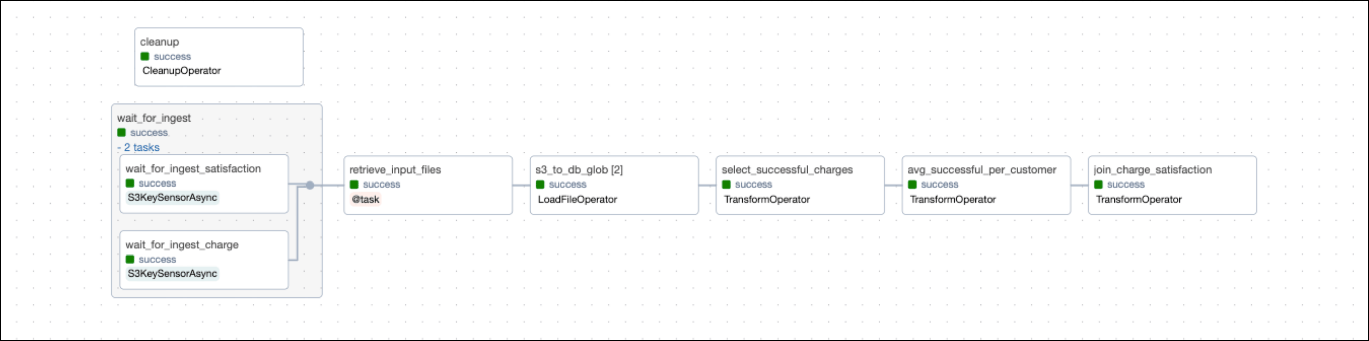
 The [`finance_elt`](https://github.com/astronomer/use-case-elt-ml-finance/blob/main/dags/finance_elt.py) DAG waits for files to land in the object storage using the [deferrable operator](/docs/learn/2.x/deferrable-operators) [S3KeySensorAsync](https://airflow.apache.org/registry/providers/amazon#amazon-s3-S3KeySensor). After the files are available, their contents are loaded to a Postgres database and transformed using operators from the [Astro Python SDK](https://astro-sdk-python.readthedocs.io/en/stable/index.html).
 The [`finance_ml`](https://github.com/astronomer/use-case-elt-ml-finance/blob/main/dags/finance_ml.py) DAG engineers machine learning features based on the last table created by the `finance_elt` DAG and then trains several models to predict the `amount_charged` column based on these features. The last task plots model results. Both model training and result plotting are mapped dynamically over a list of model classes and hyperparameters.
 ### Project code
This use case shows many core Airflow features like [datasets](/docs/learn/2.x/airflow-datasets), [dynamic task mapping](/docs/learn/2.x/dynamic-tasks), and [deferrable operators](/docs/learn/2.x/deferrable-operators). It also heavily uses the [Astro Python SDK](https://astro-sdk-python.readthedocs.io/en/stable/), an open-source package created by Astronomer to simplify DAG writing with Python functions for both ELT and ML use cases.
#### Ingestion DAG
The ingestion DAG, [`in_finance_data`](https://github.com/astronomer/use-case-elt-ml-finance/blob/main/dags/in_finance_data.py), is a helper DAG to simulate data arriving in your object storage from other sources, such as from manual uploads or through a [Kafka](/docs/learn/2.x/airflow-kafka) S3 sink.
The [script to create mock data](https://github.com/astronomer/use-case-elt-ml-finance/blob/main/include/create_mock_data.py) is located in the include folder and called inside a `@task` decorated function. Modularizing scripts in this way is a common pattern to make them accessible to several DAGs and also make your DAG files easier to read.
```python wrap theme={null}
from include.create_mock_data import generate_mock_data
# ...
@task
def generate_mock_data_task():
generate_mock_data()
# ...
generate_mock_data_task()
```
The data created in `include/mock_data` is uploaded to the object storage using a dynamically mapped [`LocalFilesystemToS3Operator`](https://airflow.apache.org/registry/providers/amazon#amazon-local_to_s3-LocalFilesystemToS3Operator). Note how the following example uses [`.expand_kwargs`](/docs/learn/2.x/dynamic-tasks#mapping-over-multiple-parameters) to map pairs of `filename` and `dest_key` keyword arguments.
```python expandable wrap theme={null}
@task
def get_kwargs():
list_of_kwargs = []
for filename in os.listdir("include/mock_data"):
if "charge" in filename:
kwarg_dict = {
"filename": f"include/mock_data/{filename}",
"dest_key": f"charge/{filename}",
}
elif "satisfaction" in filename:
kwarg_dict = {
"filename": f"include/mock_data/{filename}",
"dest_key": f"satisfaction/{filename}",
}
else:
print(
f"Skipping {filename} because it's not a charge or satisfaction file."
)
continue
list_of_kwargs.append(kwarg_dict)
return list_of_kwargs
upload_kwargs = get_kwargs()
generate_mock_data_task() >> upload_kwargs
upload_mock_data = LocalFilesystemToS3Operator.partial(
task_id="upload_mock_data",
dest_bucket=DATA_BUCKET_NAME,
aws_conn_id=AWS_CONN_ID,
replace="True",
).expand_kwargs(upload_kwargs)
```
#### ELT DAG
The ELT DAG, [`finance_elt`](https://github.com/astronomer/use-case-elt-ml-finance/blob/main/dags/finance_elt.py), waits for the deferrable [S3KeySensorAsync](https://airflow.apache.org/registry/providers/amazon#amazon-s3-S3KeySensor) operator to drop the file in the object storage. [Deferrable operators](/docs/learn/2.x/deferrable-operators) are operators that use the triggerer component to release their worker slot while they wait for a condition in an external tool to be met. This allows you to use resources more efficiently and save costs.
The two `wait_for_ingest_*` tasks are grouped in a [task group](/docs/learn/2.x/task-groups), which visually groups the tasks in the Airflow UI and allows you to pass arguments like `aws_conn_id` at the group level.
```python wrap theme={null}
@task_group(
default_args={
"aws_conn_id": AWS_CONN_ID,
"wildcard_match": True,
"poke_interval": POKE_INTERVAL,
},
)
def wait_for_ingest():
S3KeySensorAsync(
task_id="wait_for_ingest_charge",
bucket_key=f"s3://{DATA_BUCKET_NAME}/charge/*.csv",
)
S3KeySensorAsync(
task_id="wait_for_ingest_satisfaction",
bucket_key=f"s3://{DATA_BUCKET_NAME}/satisfaction/*.csv",
)
```
The `s3_to_db_glob` task uses the Astro Python SDK [`LoadFileOperator`](https://astro-sdk-python.readthedocs.io/en/stable/astro/sql/operators/load_file.html) to transfer the contents of the CSV files in the object storage directly into a table in a relational database, inferring the schema. The `s3_to_db_glob` task is dynamically mapped over two sets of `input_file` and `output` table keyword arguments to create two tables in the database.
```python wrap theme={null}
@task
def retrieve_input_files():
return [
{
"input_file": File(
path=f"s3://{DATA_BUCKET_NAME}/charge",
conn_id=AWS_CONN_ID,
filetype=FileType.CSV,
),
"output_table": Table(conn_id=DB_CONN_ID, name="in_charge"),
},
{
"input_file": File(
path=f"s3://{DATA_BUCKET_NAME}/satisfaction",
conn_id=AWS_CONN_ID,
filetype=FileType.CSV,
),
"output_table": Table(conn_id=DB_CONN_ID, name="in_satisfaction"),
},
]
input_files = retrieve_input_files()
s3_to_db_glob = LoadFileOperator.partial(
task_id="s3_to_db_glob",
).expand_kwargs(input_files)
```
Finally, the three transform tasks use the [`@aql.transform`](https://astro-sdk-python.readthedocs.io/en/stable/astro/sql/operators/transform.html) decorator of the Astro Python SDK to directly use SQL on an input table to create a new output table. For example, the second transform task ingests the temporary table created by the upstream task `select_successful_charges` and calculates the average amount charged per customer using a SQL statement.
The resulting temporary table is directly passed into the next task `join_charge_satisfaction`, which joins the average amount charged per customer with the customer satisfaction scores and creates a permanent output table called `model_satisfaction`.
```python wrap theme={null}
@aql.transform()
def avg_successful_per_customer(tmp_successful: Table) -> Table:
return """
SELECT
customer_id,
AVG(amount_captured) AS avg_amount_captured
FROM {{ tmp_successful }}
GROUP BY customer_id;
"""
# ...
# create a temporary table of successful charges from the in_charge table
tmp_successful = select_successful_charges(
Table(conn_id=DB_CONN_ID, name="in_charge")
)
# ...
# create a temporary table of average amount charged per customer
tmp_avg_successful_per_us_customer = avg_successful_per_customer(tmp_successful)
# join the average amount charged per customer with the customer satisfaction scores
# in a permanent table called model_satisfaction
join_charge_satisfaction(
tmp_avg_successful_per_us_customer,
Table(conn_id=DB_CONN_ID, name="in_satisfaction"),
output_table=Table(conn_id=DB_CONN_ID, name="model_satisfaction"),
)
```
Additionally, a [cleanup](https://astro-sdk-python.readthedocs.io/en/stable/astro/sql/operators/cleanup.html) task runs in parallel to remove the temporary tables after they are no longer needed.
#### ML DAG
Airflow [datasets](/docs/learn/2.x/airflow-datasets) let you schedule DAGs based on when a specific file or database is updated in a separate DAG. In this example, the ML DAG [`finance_ml`](https://github.com/astronomer/use-case-elt-ml-finance/blob/main/dags/finance_ml.py) is scheduled to run as soon as the `model_satisfaction` table is updated by the ELT DAG. Since the Astro Python SDK is used to update the `model_satisfaction` table, the dataset is automatically created and updated, without explicit `outlets` arguments.
The `schedule` parameter of the ML DAG uses the same `Table` definition as a dataset.
```python wrap theme={null}
@dag(
start_date=datetime(2023, 9, 1),
schedule=[Table(conn_id=DB_CONN_ID, name="model_satisfaction")],
catchup=False,
)
```
The first task of the ML DAG takes care of feature engineering. By using the [`@aql.dataframe`](https://astro-sdk-python.readthedocs.io/en/stable/astro/sql/operators/dataframe.html) decorator, the `model_satisfaction` table is ingested directly as a [pandas DataFrame](https://pandas.pydata.org/docs/reference/api/pandas.DataFrame.html).
The `feature_eng` task creates a train-test split, scales the numeric features, and one-hot encodes the categorical feature `product_type` using functions from [scikit-learn](https://scikit-learn.org/stable/index.html). The resulting sets of features and targets are returned as a dictionary of pandas DataFrames.
```python expandable wrap theme={null}
@aql.dataframe()
def feature_eng(df: pd.DataFrame):
from sklearn.model_selection import train_test_split
from sklearn.preprocessing import StandardScaler, OneHotEncoder
y = df["avg_amount_captured"]
X = df.drop(columns=["avg_amount_captured"])[
[
"customer_satisfaction_speed",
"customer_satisfaction_product",
"customer_satisfaction_service",
"product_type",
]
]
X_train, X_test, y_train, y_test = train_test_split(
X, y, test_size=0.2, random_state=42
)
# ...
scaler = StandardScaler()
X_train[numeric_columns] = scaler.fit_transform(X_train[numeric_columns])
X_test[numeric_columns] = scaler.transform(X_test[numeric_columns])
onehot_encoder = OneHotEncoder(sparse=False, drop="first")
onehot_encoder.fit(X_train[["product_type"]])
product_type_train = onehot_encoder.transform(X_train[["product_type"]])
product_type_test = onehot_encoder.transform(X_test[["product_type"]])
# ...
return {
"X_train": X_train,
"X_test": X_test,
"y_train_df": y_train_df,
"y_test_df": y_test_df,
}
# ...
feature_eng_table = feature_eng(
Table(
conn_id=DB_CONN_ID,
metadata=Metadata(schema=DB_SCHEMA),
name="model_satisfaction",
),
)
```
This DAG includes two possible paths for model training, based on whether the Airflow instance runs on [Kubernetes](https://kubernetes.io/).
Since Airflow DAGs are defined as Python code, different task definitions for different environments can be achieved by a simple if/else statement. If the environment is `prod`, the model training task runs using the [`@task.kubernetes`](/docs/learn/2.x/kubepod-operator#use-the-@task-kubernetes-decorator) decorator, which is the decorator version of the [`KubernetesPodOperator`](https://airflow.apache.org/registry/providers/cncf-kubernetes#cncf-kubernetes-pod-KubernetesPodOperator). This allows you to run your model training in a dedicated Kubernetes pod, gaining full control over the environment and resources used.
Additionally, Astro customers can use the `queue` parameter to run this task using a dedicated [worker queue](/docs/astro/configure-worker-queues) with more resources.
If the environment is `local`, a regular `@task` decorator is used.
```python expandable wrap theme={null}
if ENVIRONMENT == "prod":
# get the current Kubernetes namespace Airflow is running in
namespace = conf.get("kubernetes", "NAMESPACE")
@task.kubernetes(
image="",
in_cluster=True,
namespace=namespace,
name="my_model_train_pod",
get_logs=True,
log_events_on_failure=True,
do_xcom_push=True,
queue="machine-learning-tasks" # optional setting for Astro customers
)
def train_model_task(feature_eng_table, model_class, hyper_parameters={}):
model_results = train_model(
feature_eng_table=feature_eng_table,
model_class=model_class,
hyper_parameters=hyper_parameters,
)
return model_results
elif ENVIRONMENT == "local":
@task
def train_model_task(feature_eng_table, model_class, hyper_parameters={}):
model_results = train_model(
feature_eng_table=feature_eng_table,
model_class=model_class,
hyper_parameters=hyper_parameters,
)
return model_results
else:
raise ValueError(f"Unknown environment: {ENVIRONMENT}")
```
Both definitions of the `train_model_task` shown in the previous example call the same `train_model` function, which takes in the engineered features as well as the model class and hyperparameters as arguments. To train several models in parallel, the `train_model_task` is dynamically mapped over a list of model classes and hyperparameters. Tweak the hyperparameters to improve the model fit and add other [scikit-learn regression models](https://scikit-learn.org/stable/modules/classes.html) to the list to try them out!
```python expandable wrap theme={null}
def train_model(feature_eng_table, model_class, hyper_parameters):
from sklearn.metrics import r2_score
print(f"Training model: {model_class.__name__}")
# ...
model = model_class(**hyper_parameters)
model.fit(X_train, y_train)
y_pred_train = model.predict(X_train)
y_pred_test = model.predict(X_test)
r2_train = r2_score(y_train, y_pred_train)
r2_test = r2_score(y_test, y_pred_test)
# ...
return {
"model_class_name": model_class.__name__,
"r2_train": r2_train,
"r2_test": r2_test,
"feature_imp_coef": feature_imp_coef,
"y_train_df": y_train_df,
"y_pred_train_df": y_pred_train_df,
"y_test_df": y_test_df,
"y_pred_test_df": y_pred_test_df,
}
# ...
model_results = train_model_task.partial(
feature_eng_table=feature_eng_table
).expand_kwargs(
[
{
"model_class": RandomForestRegressor,
"hyper_parameters": {"n_estimators": 2000},
},
{"model_class": LinearRegression},
{
"model_class": RidgeCV,
"hyper_parameters": {"alphas": [0.1, 1.0, 10.0]},
},
{
"model_class": Lasso,
"hyper_parameters": {"alpha": 2.0},
},
]
)
```
Lastly, the model results are plotted using [matplotlib](https://matplotlib.org/) and [seaborn](https://seaborn.pydata.org/). The `plot_model_results` task is dynamically mapped over the list of model results to create one plot for each model trained. The plots are saved in `include/plots`.
```python expandable wrap theme={null}
@task
def plot_model_results(model_results):
# ...
fig, axes = plt.subplots(1, 2, figsize=(14, 7))
sns.scatterplot(
ax=axes[0],
x="True",
y="Predicted",
data=train_comparison,
color="black",
marker="x",
)
axes[0].plot(
[train_comparison["True"].min(), train_comparison["True"].max()],
[train_comparison["True"].min(), train_comparison["True"].max()],
"--",
linewidth=1,
color="red",
)
axes[0].grid(True, linestyle="--", linewidth=0.5)
axes[0].set_title(f"Train Set: {model_class_name}")
axes[0].text(0.1, 0.9, f"R2: {r2_train}", transform=axes[0].transAxes)
sns.scatterplot(
ax=axes[1],
x="True",
y="Predicted",
data=test_comparison,
color="black",
marker="x",
)
axes[1].plot(
[test_comparison["True"].min(), test_comparison["True"].max()],
[test_comparison["True"].min(), test_comparison["True"].max()],
"--",
linewidth=1,
color="red",
)
axes[1].grid(True, linestyle="--", linewidth=0.5)
axes[1].set_title(f"Test Set: {model_class_name}")
axes[1].text(0.1, 0.9, f"R2: {r2_test}", transform=axes[1].transAxes)
fig.suptitle("Predicted vs True Values", fontsize=16)
plt.tight_layout()
plt.savefig(f"include/plots/{model_class_name}_plot_results.png")
plot_model_results.expand(model_results=model_results)
```
Congratulations! You ran an end to end pipeline from data ingestion to model training and plotting using Airflow and the Astro Python SDK! Use this project as a blueprint to build your own data-driven pipelines.
## See also
* Documentation: [Astro Python SDK](https://astro-sdk-python.readthedocs.io/en/stable/index.html).
* Guide: [Datasets](/docs/learn/2.x/airflow-datasets).
* Guide: [Dynamic task mapping](/docs/learn/2.x/dynamic-tasks).
### Project code
This use case shows many core Airflow features like [datasets](/docs/learn/2.x/airflow-datasets), [dynamic task mapping](/docs/learn/2.x/dynamic-tasks), and [deferrable operators](/docs/learn/2.x/deferrable-operators). It also heavily uses the [Astro Python SDK](https://astro-sdk-python.readthedocs.io/en/stable/), an open-source package created by Astronomer to simplify DAG writing with Python functions for both ELT and ML use cases.
#### Ingestion DAG
The ingestion DAG, [`in_finance_data`](https://github.com/astronomer/use-case-elt-ml-finance/blob/main/dags/in_finance_data.py), is a helper DAG to simulate data arriving in your object storage from other sources, such as from manual uploads or through a [Kafka](/docs/learn/2.x/airflow-kafka) S3 sink.
The [script to create mock data](https://github.com/astronomer/use-case-elt-ml-finance/blob/main/include/create_mock_data.py) is located in the include folder and called inside a `@task` decorated function. Modularizing scripts in this way is a common pattern to make them accessible to several DAGs and also make your DAG files easier to read.
```python wrap theme={null}
from include.create_mock_data import generate_mock_data
# ...
@task
def generate_mock_data_task():
generate_mock_data()
# ...
generate_mock_data_task()
```
The data created in `include/mock_data` is uploaded to the object storage using a dynamically mapped [`LocalFilesystemToS3Operator`](https://airflow.apache.org/registry/providers/amazon#amazon-local_to_s3-LocalFilesystemToS3Operator). Note how the following example uses [`.expand_kwargs`](/docs/learn/2.x/dynamic-tasks#mapping-over-multiple-parameters) to map pairs of `filename` and `dest_key` keyword arguments.
```python expandable wrap theme={null}
@task
def get_kwargs():
list_of_kwargs = []
for filename in os.listdir("include/mock_data"):
if "charge" in filename:
kwarg_dict = {
"filename": f"include/mock_data/{filename}",
"dest_key": f"charge/{filename}",
}
elif "satisfaction" in filename:
kwarg_dict = {
"filename": f"include/mock_data/{filename}",
"dest_key": f"satisfaction/{filename}",
}
else:
print(
f"Skipping {filename} because it's not a charge or satisfaction file."
)
continue
list_of_kwargs.append(kwarg_dict)
return list_of_kwargs
upload_kwargs = get_kwargs()
generate_mock_data_task() >> upload_kwargs
upload_mock_data = LocalFilesystemToS3Operator.partial(
task_id="upload_mock_data",
dest_bucket=DATA_BUCKET_NAME,
aws_conn_id=AWS_CONN_ID,
replace="True",
).expand_kwargs(upload_kwargs)
```
#### ELT DAG
The ELT DAG, [`finance_elt`](https://github.com/astronomer/use-case-elt-ml-finance/blob/main/dags/finance_elt.py), waits for the deferrable [S3KeySensorAsync](https://airflow.apache.org/registry/providers/amazon#amazon-s3-S3KeySensor) operator to drop the file in the object storage. [Deferrable operators](/docs/learn/2.x/deferrable-operators) are operators that use the triggerer component to release their worker slot while they wait for a condition in an external tool to be met. This allows you to use resources more efficiently and save costs.
The two `wait_for_ingest_*` tasks are grouped in a [task group](/docs/learn/2.x/task-groups), which visually groups the tasks in the Airflow UI and allows you to pass arguments like `aws_conn_id` at the group level.
```python wrap theme={null}
@task_group(
default_args={
"aws_conn_id": AWS_CONN_ID,
"wildcard_match": True,
"poke_interval": POKE_INTERVAL,
},
)
def wait_for_ingest():
S3KeySensorAsync(
task_id="wait_for_ingest_charge",
bucket_key=f"s3://{DATA_BUCKET_NAME}/charge/*.csv",
)
S3KeySensorAsync(
task_id="wait_for_ingest_satisfaction",
bucket_key=f"s3://{DATA_BUCKET_NAME}/satisfaction/*.csv",
)
```
The `s3_to_db_glob` task uses the Astro Python SDK [`LoadFileOperator`](https://astro-sdk-python.readthedocs.io/en/stable/astro/sql/operators/load_file.html) to transfer the contents of the CSV files in the object storage directly into a table in a relational database, inferring the schema. The `s3_to_db_glob` task is dynamically mapped over two sets of `input_file` and `output` table keyword arguments to create two tables in the database.
```python wrap theme={null}
@task
def retrieve_input_files():
return [
{
"input_file": File(
path=f"s3://{DATA_BUCKET_NAME}/charge",
conn_id=AWS_CONN_ID,
filetype=FileType.CSV,
),
"output_table": Table(conn_id=DB_CONN_ID, name="in_charge"),
},
{
"input_file": File(
path=f"s3://{DATA_BUCKET_NAME}/satisfaction",
conn_id=AWS_CONN_ID,
filetype=FileType.CSV,
),
"output_table": Table(conn_id=DB_CONN_ID, name="in_satisfaction"),
},
]
input_files = retrieve_input_files()
s3_to_db_glob = LoadFileOperator.partial(
task_id="s3_to_db_glob",
).expand_kwargs(input_files)
```
Finally, the three transform tasks use the [`@aql.transform`](https://astro-sdk-python.readthedocs.io/en/stable/astro/sql/operators/transform.html) decorator of the Astro Python SDK to directly use SQL on an input table to create a new output table. For example, the second transform task ingests the temporary table created by the upstream task `select_successful_charges` and calculates the average amount charged per customer using a SQL statement.
The resulting temporary table is directly passed into the next task `join_charge_satisfaction`, which joins the average amount charged per customer with the customer satisfaction scores and creates a permanent output table called `model_satisfaction`.
```python wrap theme={null}
@aql.transform()
def avg_successful_per_customer(tmp_successful: Table) -> Table:
return """
SELECT
customer_id,
AVG(amount_captured) AS avg_amount_captured
FROM {{ tmp_successful }}
GROUP BY customer_id;
"""
# ...
# create a temporary table of successful charges from the in_charge table
tmp_successful = select_successful_charges(
Table(conn_id=DB_CONN_ID, name="in_charge")
)
# ...
# create a temporary table of average amount charged per customer
tmp_avg_successful_per_us_customer = avg_successful_per_customer(tmp_successful)
# join the average amount charged per customer with the customer satisfaction scores
# in a permanent table called model_satisfaction
join_charge_satisfaction(
tmp_avg_successful_per_us_customer,
Table(conn_id=DB_CONN_ID, name="in_satisfaction"),
output_table=Table(conn_id=DB_CONN_ID, name="model_satisfaction"),
)
```
Additionally, a [cleanup](https://astro-sdk-python.readthedocs.io/en/stable/astro/sql/operators/cleanup.html) task runs in parallel to remove the temporary tables after they are no longer needed.
#### ML DAG
Airflow [datasets](/docs/learn/2.x/airflow-datasets) let you schedule DAGs based on when a specific file or database is updated in a separate DAG. In this example, the ML DAG [`finance_ml`](https://github.com/astronomer/use-case-elt-ml-finance/blob/main/dags/finance_ml.py) is scheduled to run as soon as the `model_satisfaction` table is updated by the ELT DAG. Since the Astro Python SDK is used to update the `model_satisfaction` table, the dataset is automatically created and updated, without explicit `outlets` arguments.
The `schedule` parameter of the ML DAG uses the same `Table` definition as a dataset.
```python wrap theme={null}
@dag(
start_date=datetime(2023, 9, 1),
schedule=[Table(conn_id=DB_CONN_ID, name="model_satisfaction")],
catchup=False,
)
```
The first task of the ML DAG takes care of feature engineering. By using the [`@aql.dataframe`](https://astro-sdk-python.readthedocs.io/en/stable/astro/sql/operators/dataframe.html) decorator, the `model_satisfaction` table is ingested directly as a [pandas DataFrame](https://pandas.pydata.org/docs/reference/api/pandas.DataFrame.html).
The `feature_eng` task creates a train-test split, scales the numeric features, and one-hot encodes the categorical feature `product_type` using functions from [scikit-learn](https://scikit-learn.org/stable/index.html). The resulting sets of features and targets are returned as a dictionary of pandas DataFrames.
```python expandable wrap theme={null}
@aql.dataframe()
def feature_eng(df: pd.DataFrame):
from sklearn.model_selection import train_test_split
from sklearn.preprocessing import StandardScaler, OneHotEncoder
y = df["avg_amount_captured"]
X = df.drop(columns=["avg_amount_captured"])[
[
"customer_satisfaction_speed",
"customer_satisfaction_product",
"customer_satisfaction_service",
"product_type",
]
]
X_train, X_test, y_train, y_test = train_test_split(
X, y, test_size=0.2, random_state=42
)
# ...
scaler = StandardScaler()
X_train[numeric_columns] = scaler.fit_transform(X_train[numeric_columns])
X_test[numeric_columns] = scaler.transform(X_test[numeric_columns])
onehot_encoder = OneHotEncoder(sparse=False, drop="first")
onehot_encoder.fit(X_train[["product_type"]])
product_type_train = onehot_encoder.transform(X_train[["product_type"]])
product_type_test = onehot_encoder.transform(X_test[["product_type"]])
# ...
return {
"X_train": X_train,
"X_test": X_test,
"y_train_df": y_train_df,
"y_test_df": y_test_df,
}
# ...
feature_eng_table = feature_eng(
Table(
conn_id=DB_CONN_ID,
metadata=Metadata(schema=DB_SCHEMA),
name="model_satisfaction",
),
)
```
This DAG includes two possible paths for model training, based on whether the Airflow instance runs on [Kubernetes](https://kubernetes.io/).
Since Airflow DAGs are defined as Python code, different task definitions for different environments can be achieved by a simple if/else statement. If the environment is `prod`, the model training task runs using the [`@task.kubernetes`](/docs/learn/2.x/kubepod-operator#use-the-@task-kubernetes-decorator) decorator, which is the decorator version of the [`KubernetesPodOperator`](https://airflow.apache.org/registry/providers/cncf-kubernetes#cncf-kubernetes-pod-KubernetesPodOperator). This allows you to run your model training in a dedicated Kubernetes pod, gaining full control over the environment and resources used.
Additionally, Astro customers can use the `queue` parameter to run this task using a dedicated [worker queue](/docs/astro/configure-worker-queues) with more resources.
If the environment is `local`, a regular `@task` decorator is used.
```python expandable wrap theme={null}
if ENVIRONMENT == "prod":
# get the current Kubernetes namespace Airflow is running in
namespace = conf.get("kubernetes", "NAMESPACE")
@task.kubernetes(
image="",
in_cluster=True,
namespace=namespace,
name="my_model_train_pod",
get_logs=True,
log_events_on_failure=True,
do_xcom_push=True,
queue="machine-learning-tasks" # optional setting for Astro customers
)
def train_model_task(feature_eng_table, model_class, hyper_parameters={}):
model_results = train_model(
feature_eng_table=feature_eng_table,
model_class=model_class,
hyper_parameters=hyper_parameters,
)
return model_results
elif ENVIRONMENT == "local":
@task
def train_model_task(feature_eng_table, model_class, hyper_parameters={}):
model_results = train_model(
feature_eng_table=feature_eng_table,
model_class=model_class,
hyper_parameters=hyper_parameters,
)
return model_results
else:
raise ValueError(f"Unknown environment: {ENVIRONMENT}")
```
Both definitions of the `train_model_task` shown in the previous example call the same `train_model` function, which takes in the engineered features as well as the model class and hyperparameters as arguments. To train several models in parallel, the `train_model_task` is dynamically mapped over a list of model classes and hyperparameters. Tweak the hyperparameters to improve the model fit and add other [scikit-learn regression models](https://scikit-learn.org/stable/modules/classes.html) to the list to try them out!
```python expandable wrap theme={null}
def train_model(feature_eng_table, model_class, hyper_parameters):
from sklearn.metrics import r2_score
print(f"Training model: {model_class.__name__}")
# ...
model = model_class(**hyper_parameters)
model.fit(X_train, y_train)
y_pred_train = model.predict(X_train)
y_pred_test = model.predict(X_test)
r2_train = r2_score(y_train, y_pred_train)
r2_test = r2_score(y_test, y_pred_test)
# ...
return {
"model_class_name": model_class.__name__,
"r2_train": r2_train,
"r2_test": r2_test,
"feature_imp_coef": feature_imp_coef,
"y_train_df": y_train_df,
"y_pred_train_df": y_pred_train_df,
"y_test_df": y_test_df,
"y_pred_test_df": y_pred_test_df,
}
# ...
model_results = train_model_task.partial(
feature_eng_table=feature_eng_table
).expand_kwargs(
[
{
"model_class": RandomForestRegressor,
"hyper_parameters": {"n_estimators": 2000},
},
{"model_class": LinearRegression},
{
"model_class": RidgeCV,
"hyper_parameters": {"alphas": [0.1, 1.0, 10.0]},
},
{
"model_class": Lasso,
"hyper_parameters": {"alpha": 2.0},
},
]
)
```
Lastly, the model results are plotted using [matplotlib](https://matplotlib.org/) and [seaborn](https://seaborn.pydata.org/). The `plot_model_results` task is dynamically mapped over the list of model results to create one plot for each model trained. The plots are saved in `include/plots`.
```python expandable wrap theme={null}
@task
def plot_model_results(model_results):
# ...
fig, axes = plt.subplots(1, 2, figsize=(14, 7))
sns.scatterplot(
ax=axes[0],
x="True",
y="Predicted",
data=train_comparison,
color="black",
marker="x",
)
axes[0].plot(
[train_comparison["True"].min(), train_comparison["True"].max()],
[train_comparison["True"].min(), train_comparison["True"].max()],
"--",
linewidth=1,
color="red",
)
axes[0].grid(True, linestyle="--", linewidth=0.5)
axes[0].set_title(f"Train Set: {model_class_name}")
axes[0].text(0.1, 0.9, f"R2: {r2_train}", transform=axes[0].transAxes)
sns.scatterplot(
ax=axes[1],
x="True",
y="Predicted",
data=test_comparison,
color="black",
marker="x",
)
axes[1].plot(
[test_comparison["True"].min(), test_comparison["True"].max()],
[test_comparison["True"].min(), test_comparison["True"].max()],
"--",
linewidth=1,
color="red",
)
axes[1].grid(True, linestyle="--", linewidth=0.5)
axes[1].set_title(f"Test Set: {model_class_name}")
axes[1].text(0.1, 0.9, f"R2: {r2_test}", transform=axes[1].transAxes)
fig.suptitle("Predicted vs True Values", fontsize=16)
plt.tight_layout()
plt.savefig(f"include/plots/{model_class_name}_plot_results.png")
plot_model_results.expand(model_results=model_results)
```
Congratulations! You ran an end to end pipeline from data ingestion to model training and plotting using Airflow and the Astro Python SDK! Use this project as a blueprint to build your own data-driven pipelines.
## See also
* Documentation: [Astro Python SDK](https://astro-sdk-python.readthedocs.io/en/stable/index.html).
* Guide: [Datasets](/docs/learn/2.x/airflow-datasets).
* Guide: [Dynamic task mapping](/docs/learn/2.x/dynamic-tasks).